
The small amount of work we do by rubbing provides the energy necessary for the electrons to make it over the necessary activation 'hump.'
Interactions between Materials &
Franklin's One Fluid Model
A Twentieth Century Explanation
Properties of Charge
Coulomb's Law
The Electric Field
Gauss's Law
Metals
Dipoles
Correlation
to your Textbook
| bakelite | wool | glass | silk | |
| bakelite | R | A | A | R |
| wool | A | R | R | A |
| glass | A | R | R | A |
| silk | R | A | A | R |
| bakelite (-) | wool (+) | glass | silk | |
| bakelite (-) | R | A | A | R |
| wool (+) | A | R | R | A |
| glass | A | R | R | A |
| silk | R | A | A | R |
Then, we see that the glass would have to be positive to attract the
negative bakelite. We might then predict that the (+)
glass
would then repel the (+) wool (that is , that positive charge repels
positive
charge, or more generally that like charges repel), and this is
in fact consistent with our observations. We predict that the
silk
is negative, since it was attracted to the (+) glass, and we finish off
by predicting the rest of the interactions:
bakelite (-) should repel silk (-) - correct
wool (+) should attract silk (-) - correct.
We need to verify this model for many more combinations of materials,
but we may well have assured ourselves that it is a valid working
model.
Now we have two working models: one which requires two types of charges
and two rules, and another which has an infinite number of types of
charges
(silk-type, wool- type, et c.) and an infinite number of
rules.
Which should we accept as correct? We employ Occam's Razor
to assume that the simpler of two equally valid explanations is the
correct
one.

In the demos we did in the previous section, we always charged the
objects
by rubbing them together. This took charge from one object and
deposited
it on the other; which way the charge goes depends entirely on energy
considerations.
We see that the electrons are almost always what moves, since they are
one thousand to ten million times easier to remove from the outer edges
of an atom than are the protons deep in the nucleus. Once
removed,
they are 2000 times easier to move around, due to their smaller
mass. For example, when we rubbed the wool on the bakelite,
electrons were
transferred from the wool to the bakelite, causing an excess of
electrons
on the bakelite, making it negatively charged, and a deficit of
electrons
on the wool, rendering it positively charged. This occurred
because
the electrons have a slightly lower energy when on the Bakelite than
when
on the wool.
The small amount of work we do by rubbing provides the energy necessary
for the electrons to make it over the necessary activation 'hump.'
Here is an example to consider: anti-matter does
exist
outside of Star TrekR. For each sub-atomic
particle
of matter, there is an anti-particle which is identical in every way
except
that it has the opposite charge. When anti-pairs contact one
another,
both are destroyed (annihilated) and the energy is carried away
in electro-magnetic radiation, usually gamma rays.
Consider
this reaction: p+ + p- = 2 go.
Is charge conserved in this reaction?
We also say that charge is quantized, by which we mean that there is a smallest non-zero amount of charge possible (given the symbol e), and that all charges are integer multiples of that fundamental charge (i.e., 0, +/-e, +/-2e, +/-3e, et c.). This is shown by the famous Millikan oil drop experiment (Yes, O.K., earlier work by Faraday suggested quantization). We find that the fundamental charge amount corresponds to the charge on a proton, which is equal although opposite to the charge on the electron; since the electron was only discovered in 1899 and the proton after that, this is a recent discovery. Before the discovery of this fundamental quantity, charges were measured in larger, more convenient, but completely arbitrary units called coulombs; 1e = 1.6x10⁻¹⁹ C, or 1C = 6x10+18 e.
As an aside, there is a theory that there are particles called quarks
that have charges less than e (+/- 1/3e
or
+/-
2/3e).
It is thought that combinations of quarks make up protons, neutrons,
and
many other particles (but not electrons). This model has been
very
successful in predicting the results of various reactions between
particles,
however, individual quarks have never been seen. For the purposes
of this class, they do not exist.
How should we approach situations in which there are more than two charges? We asserted in Section 4 of the first semestre that forces can be super-imposed, that is, added as vectors. So we find the force exerted on any given charge by each of the other charged, then add.
Example:
Consider two identical positive charges q which are separated by a
distance R; a third, negative charge of the same magnitude is located
exactly between the other two. Find the net force
a) on the leftt hand charge.
b) on the centre charge.
Example:
Three charges are arranged as described below:
| Charge | x co-ordinate | y co-ordinate | |
| Q1 | -2 nC | 0 | -0.1 m |
| Q2 | +5 nC | 0 | 0 |
| Q3 | +6 nC | +0.3 m | 0 |
Newton worked out, based on Kepler's Laws of Planetary Motion, that
two masses M1 and M2, separated by distance r,
will
attract each other with (mutual) forces whose (equal) magnitudes are
given
by
F = GM1M2/r2.
Here, G is a constant used just to make the units work out and is equal
to 6.67x10⁻¹¹ Nm2/kg2. This
relationship
is Newton's Law of Universal Gravitation.
Let's check it out. We already know that the weight of an object
near the earth's surface is W = g m, and that this same force is
described
by W = GmMEARTH/REARTH2. So,
g m = GmMEARTHREARTH2.
g = GMEARTH/REARTH2 = 6.67x10-11*6x1024/[6.4x106]2
= 9.77 N/kg, about what we expected.
Let's consider a fixed charge +Q in space. If we bring a small
test charge +q near to +Q, it will be repelled by a force given by:
F = keQq/r2.

Let's define the electric field of charge +Q at some location
as the force per unit charge that +Q would exert on a test charge qTEST
put in that location:
E = limq ->0 F/qTEST.
we note that since F is a vector, so is E. The
units of electric field are newtons per coulomb (N/C).
So, if we place +qTEST at various locations around +Q and
find the direction of E at each, we see that the field from +Q
points
radially outward from +Q. Can we find the magnitude? The
force
between the charges is F = keQqTEST/r2,
so the field is:
E = F/q = [keQqTEST/r2]/qTEST
= keQ/r2 radially outward.
| NOTE: This relationship is valid only for the field produced by a point charge, since the force is based on the interaction between two point charges. The fields produced by other shapes may well have very different dependences. |
How do we find the field from more complicated distributions of
charge?
If the distribution is made up of a collection of point charges, then
we
find the field at some point P by adding the individual fields (as
vectors,
remember) due to the individual charges.
We did several examples in class.
What if the distribution of charge is not composed of discreet points, but rather is continuous. In principle, the method is the same as in the last paragraph, but the execution of that method usually requires calculus. We shall see in the next section a method which will allow us to find E for certain highly symmetrical distributions of charge. However, there are a few special shapes for which calculus is not required.
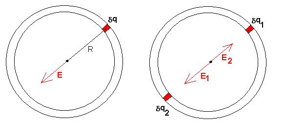
Example:
Consider a circular ring of radius R that carries a uniformly
distributed
charge Q. What is the electric field at the centre of the ring?

Now let's look at a different shape to see if this relationship
holds.
If we imagine that the sphere is cut into two hemispheres, the quantity
EA will be 2pkeQ for each
half.
Let's shrink one half of the sphere to radius R.

Since EA is independent of the radius, each 'half' sphere will still
have flux 2pkeQ. However,
there
is now a third surface to worry about, the flat annular surface which
connects
the edges of the hemispheres (shown in green). Here, the area A =
p[R2
- R2] and the
field
E is certainly not zero (and not even constant!), and so the total flux
(as initially defined) is greater than 4pkeQ.
Rather than give up, can we somehow save our notion?
Notice that the electric field on the hemispherical portions is
perpendicular
to the surfaces, but that the field along the annulus is parallel to
the
surface. If we were to change our definition of flux to EperpA,
the contribution from the annulus would be zero and the total would be
fE = (Eperp)1A1
+ (Eperp)2A2 + (Eperp)3A3=
[keQ/R2]*2pR2
+ [keQ/R2]*2pR2
+ [0]*p[R2 - R2]
= 2pkeQ + 2pkeQ
+ 0 = 4pkeQ once again.
Yippee!
Now, what if the surface surrounding +Q is of any arbitrary
shape?
We can always approximate the surface's shape to an arbitrary degree of
accuracy with a series of spherical sections with their centers at +Q.

This gives us two types of individual surfaces dAi
to work with: the curved sections for which E is still perpendicular
and
for which the flux is (Eperp)idAi,
and the sides of the sections for which E runs along the surfaces and
for
which the flux contribution is zero (Eperp = 0). The
total
flux through such a surface should be the sum of the fluxes through
each
small surface, or
fE = Si
(Eperp)idAi.
We can then push and pull the spherical sections until they form a
sphere again, remembering that the flux through each individual section
does not change as the section is moved, since those that move closer
to
+Q get smaller areas but have E-field strengths which increase by the
same
factor that the areas decrease. In the end, we have a sphere with
flux 4pkeQ again. So, we
can
safely assert that the flux from +Q through any closed surface
surrounding
it must be 4pkeQ, and that the
total
flux through that surface can be found from the sums of the fluxes
through
the component parts of the surface.
What if there is more than one charge? The total field at any
point is the vector sum of the fields due to the individual charges Q1
and Q2:
Etotal = E1 + E2.
As a result, we can also say that the perpendicular component of the
total field is the sum of the perpendicular components of the fields
due
to each charge:
(Etotal)perp = E1perp + E2perp.
We can write that
ftotal = Si
[(Etotal)perp]idAi
= S [[E1perp]i
+ [E2perp]i]dAi
= S [E1perp]idAi
+ S [E2perp]idAi
= 4pkeQ1 + 4pkeQ2
= 4pke(Q1 + Q2),
which we can generalize to as many charges as you like.
What if the charge inside is negative? Hey, good question,
shows
you're thinking. Suppose that I put a positive charge +Q and a
smaller
negative charge (-q) inside a closed surface, close to each other but
far
from the surface. It should be pretty clear that the total
electric
field at any point on the surface will be reduced from the value it
would
have had when only the positive charge was there, since the outward
pointing
field from +Q will be partially if not completely canceled by the
inward
pointing field from (-q). This reduction in the magnitude of Etotal
will correspondingly reduce the total flux
ftotal =
Si
[(Etotal)perp]idAi,
and Etotal is smaller than it was). From the last
section,
we showed that the total flux should be the sum of the flux due to +Q
alone
and the flux due to (-q) alone. Since adding the flux from (-q) reduces
the total flux, that number must be negative. So we
define
the flux due to a negative charge to be negative. Now the field
at
the surface doesn't know or care what causes it, and the flux
calculation
will be the same regardless, so we generalize the result to say that
flux
due to any E-line going from the outside of the surface to the
inside
is counted as negative flux.
What if the charge is outside of the surface? In that case,
the
total flux through that surface due to that charge is zero. Once
again, any shape closed surface can be approximated to arbitrary
accuracy
with the spherical sections centered on the charge. As above, I
can
then push and pull the sections to get a nice double spherical surface
shape. Since the quantity EA has already been shown to be
independent
of the distance from the charge, and since we have just defined the
flux
from E-lines entering a surface to be negative while the flux from
those
leaving a surface are positive, and since the fluxes through those side
portions of the sections are zero since Eperp = 0, we see
that
the total flux through this surface due to an exterior charge is zero.

At this point, we have arrived at something useful.
Gauss's Law for Electricity: The net electric flux through a closed surface is proportional to the net charge inside the surface.
The flux is defined as
ftotal = Si
[Eperp]i
dAi
and it is calculated by looking at each little piece of area, dAi,
multiplying by the component of Ei that is perpendicular to
the area, assigning a sign (positive if E points from the inside of the
surface to the outside, negative if the reverse is so), and adding up
all
the contributions from each area. When this is done, the total
should
equal 4pkeQnet enclosed.
Here, we introduce a new and sometimes more convenient constant, eo,
the permittivity of free space. The value of eo
is 1/[4pke]. So, finally,
we
have that
ftotal = Si
[Eperp]i
dAi
= [Qnet enclosed]/eo.
Let's now use Gauss's Law to find the electric field due to some very special, highly symmetric distributions of charge. The symmetry is important since, although Gauss's law is always true, it is not always possible to work it backwards to find E.
Uniform Infinite Straight Line Charge:
Consider a straight, infinitely long wire which carries a uniform linear
charge density l = Q/L.
Let's get an idea what the E-field looks like at some point P a
distance
R from the line charge

Consider some small bit of charge Q1, which will cause a
field E1 at P. For every one of these charges, there
is
another charge Q2 the same distance away, but on the other
side
of P. The fields E1 and E2 will have the
same
magnitudes, since P is the same distance r from each charge. In
addition,
the horizontal components of the two fields will be the same (although
in opposite directions) because the angles q
are the same. The resultant E-field from Q1 and Q2
is directly away from the line charge. This is true for any pair
of charges, and also for the single charge directly under Point P, so
the
total E-field at Point P must be radially outward perpendicular to the
wire. What's more, the magnitude of E is the same for any point
distance
R from the wire, since the argument can be repeated at any spot along
the
wire.
Now, in order to use Gauss's law, we need a gaussian surface
over which to find the flux. Since the surface is imaginary, we
can
pick one which will minimize the difficulty of the calculations we must
do while still delivering the result we want. In general, we
should
pick a surface such that either:
1) the electric field runs along the surface (or part of a surface)
so that the perpendicular component of E is zero and the contribution
to
the flux is zero, or
2) the electric field along a surface (or part of a surface) is
constant
in magnitude and, if possible, perpendicular to the surface, so that S
Eperp dA = EA.
Choose the gaussian surface to be a cylinder of variable radius R
and
length L, co-axial with the wire. The surface can be considered
to
comprise three individual surfaces, the circular end caps and the
curved
section connecting them.

Gauss's Law: for a closed surface, fE
= Si [Eperp]idAi
= 4pkeQenclosed
The total flux is the sum of the
fluxes through each part of the surface:
fE = Sleft
cap [Eperp]i dAi
+ Sright cap [Eperp]idAi
+ Scurved part [Eperp]idAi
In that case, the first two terms are zero, since the field runs along
the surfaces, not perpendicular to them. On the curved surface,
however,
E is perpendicular to the gaussian surface everywhere, so Eperp
= E and
Scurved part [Eperp]idAi
= S Ei dAi
We said above that E is constant in magnitude for any given radius
from
the centre, so this is true everywhere on the curved surface (Ei
= E), so
Scurved part Ei dAi
= E Scurved partdAi
= EA = E 2pRL = 4pkeQenclosed
Solve for E:
E = 2keQencl/LR = 2ke(Qencl/L)/R
= 2ke(l)/R
(radially outward if l is positive,
radially
inward if l is negative.)
Note that L dropped out of the result. This is very
important.
Why?
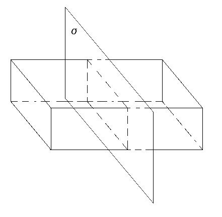
Exactly what it sounds like: a flat sheet that extends infinitely in
four directions. We define s as
the
amount of charge per unit area:
s = Q/A
We need to get some idea what the E-field looks like before we
start.
Use an argument similar to the one outlined above, or use a symmetry
argument
(done in class) to see that the field must be straight away from the
sheet
(or towards it, if s is negative).
Also,
the magnitude must be the same at any given distance from the sheet, on
either side. Pick a gaussian surface in the shape of a
rectangular box (with six
sides, top, bottom, left, right, front, back), positioned symmetrically
on the sheet, as shown in the figure.
Start with Gauss's Law: fE
= Si [Eperp]idAi
= 4pkeQenclosed
for a closed surface. Then,
fE = StopEperpdAtop
+
SbotEperpdAbot
+ SfrontEperpdAfront
+ SbackEperpdAback
+ SleftEperpdAleft
+ SrightEperpdAright.
Since E is perpendicular to
the sheet of charge, it is along the
top,
bottom, front, and back surfaces, so that there,
Eperpendicular = 0.
Then, we're left with
fE = Sleft
Eperp dAleft + Sright
Eperp dAright
For the same reason, on the left and right surfaces, E = Eperpendicular,
so that
fE = Sleft
E dA + Sright
E
dA.
Also, E is a constant along each of the right and left hand surfaces
and equal in magnitude along both, and the right and left hand sides
are
the same area as the area of the sheet enclosed by the gaussian
surface,
so
fE = E SleftdA
+ E SrightdA
= 2 EA
By Gauss's law, fE = 4pkeQenclosed
= 4pkesA.
So, 2EA = 4pkesA.
The area cancels out, as we know it should, so that we obtain
E = 2pkes
=
s/2eo.
So, the electric field of an infinite, flat, uniformly charged sheet
is constant (althoughthe direction reverses on each side).
Here, we introduce a new and sometimes more convenient constant, eo,
the permittivity of free space. The value of eo
is 1/[4pke] = 9x10-12
in SI units.
Maxwell developed the notion of the electric field line.
Let's see if we can make some connections to what we've done previously
to see if
we can suss out any information from their appearance. Consider
the
point charge with a radially outward field of magnitude E = keQ/r2
and
the infinite flat sheet with a field of parallel lines with constant
magnitude:

We note that in Region A, the lines are close together and the field
is strong, while in Region B the lines are far apart and the field is
weak.
This correlation seems fine and is consistent with the other example:
lines
which stay evenly separated (Regions C & D) represent constant
field
strength.
Following through on this, we can also say that the electric
flux
through a surface is proportional to the number of field lines passing
through it. For example, we argued that the flux through a
spherical
section due to a point charge remained constant regardless of r, since
the field strength and the area both have r2 terms which
then
cancel in their product, while we can easily see that the number of
lines
through each surface is also the same.

Since arbitrary shapes of charge can be approximated by a collection
of point charges, this should be true for any shape of charge.
Consider a block of metal; the distributions of electrons and
protons
are fairly uniform, even to just above the atomic scale (Figure A).
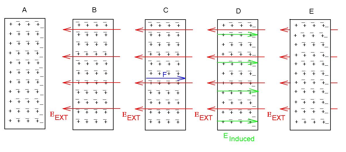
Let's place this block of metal in an external electric field, EEXT
(Figure B, EEXT is shown in red).
The electrons will experience an electric force (qE) to the
left (Figure C, the force is shown in blue), and since they are free to
move, they will start to do so toward
the rigthhand surface of the metal (they can't go any farther than
that).
The protons will experience a force to the left, but each is about
2000
times heavier than the electrons, there are 10 to 100 times as many of
them as there are free electrons (plus the neutrons too!), each is
locked
up inside of an atom, and the atoms are linked to each other in a
strong
lattice structure, so that we might think of them as composing a
single
large object, which in turn has macroscopic forces acting from, for
example,
the table on which the block sits; it's safe to say that the net force
on each proton is about zero, so they don't move.
As the electrons move rightward, the separation of charge gives rise
to an internal electric field, EINT (Figure D,
induced field shown in green), which points
from
the excess positive charge on the left toward the excess negative
charge
on the right. The net field inside the metal is the vector sum of
EEXT
and EINT, which has a magnitude of (roughly)
ENET = EEXT - EINT.
Since there is still a net field in the metal, even more electrons
will travel to the left surface, thus increasing the internal fireld
and
decreasing the net field. When does this stop?
So, we see that the electric field inside a conductor in equilibrium must be zero (Figure E); if it were not, then charges would arrange themselves until it is. Do not be surprised when I qualify this statement in a week or so.
The same argument can be applied to the electric field at the
surface
of a metal. Consider an external field which has a component
perpendicular
to the metal's surface and another along the metal's surface; since
charge
can move along the syrface, they will once again re-arrange themselves
and produce their own field parallel to the surface until the total
field
has no net component in that direction. So, we can also say that
the electric field at the surface of a conductor in equilibrium
must
be perpendicular to that surface.
Example 1:
Consider a metal sphere of radius R which has a charge 3Qo.
Where does that charge reside?
Example 2:
Consider a hollow conducting sphere (inner radius R1
and outer radius R2) with a total charge -3Qo.
Now, place a point charge +2Qo at the centre of the hollow
sphere.
What charge will be on the inner and outer surfaces of the sphere?
What does the electric field look like? Again consider a
concentric
gaussian surface of variable radius r.
For 0 < r < R1, QENCLOSED = +2Qo,
so E = 2kQo/r2 outward.
For R1< r < R2, E = 0 (inside metal).
For r > R2, QENCLOSED = +2Qo
+ (-2Qo) + (-Qo) = -Qo, so E = kQo/r2
inward.
Example 3:

Consider an infinitely long straight cylinder (radius R1)
of charge with uniform density, that is, the charge is distributed
evenly
throughout the cylinder. Let the linear charge density be
l1.
Let a thin cylindrical shell of radius R2 and with linear
charge
density l2
be co-axial with it.
Find the electric field everywhere.
Draw a gaussian surface as a cylinder (variable radius r and length
L) co-axial with the real cylinders, and make use of the result of the
derivation above for the infinitely long straight wire: E = 2kelENC/r.
For r > R2, both l1
and l2 are enclosed, so E = 2k(l1
+ l2)/r.
For R1 < r < R2, only l1
is enclosed, so E = 2kl1/r.
For 0 < r < R1, only part of the charge on
the central cylinder will be enclosed; we need to figure out how
much.
If the charge is distributed evenly within the cylinder, then the
fraction
of charge enclosed by the gaussian surface is the same as the fraction
of the volume enclosed:
lENC/l1
= pr2L/pR12L,
so that
lENC = l1r2/R12.
Substituting gives
E = 2klENC/r = 2k[l1r2/R12]/r
= 2kl1r/R12.
Example 4:
A point charge of +3Qo is located at the centre of a hollow
sphere (inner radius R1, outer radius R2) that
has
a uniform charge density throughout and a total charge of +Qo.
Find the electric field everywhere.

There is some potential energy associated
with
the dipole, since the kinetic energy of this motion had to come from
somewhere
(we can think of the source either as PE or as the work done by
the electric force, but never as both). That PE is
PEdipole = -pEcosq p,E;
let's see if we can derive this result.
Start with the dipole arranged such that (q
p,E
)o
is 90o.

Now, let the dipole rotate to an arbitrary angle q
p,E.

To calculate the work done by the electric force on, say, the positive
charge, we need only consider the displacement in the direction of the
force, which will be [L/2]cosq p,E.
The work done is then
[F+][L/2]cosqp,E =
[qE L/2]cosqp,E = 1/2
[qL E] cosqp,E = 1/2
pE cosqp,E.
A similar amount of work is done on the negative charge, so that the
total work is
WE-field = pE cosqp,E.
But, we defined the change in PE to be
DPEdipole = - WE-Field
= - pE cosqp,E.
Now, if we set the PE to zero when qp,E
=
90o (and why not?), then we have our result, that
PEdipole = - pE cosqp,E.