Section 2-6 - Magnetic Induction & Friends
Faraday's
Law of Induction
& Lenz's Law
Self Inductance
Mutual Inductance
RC Circuits
LR Circuits
Correlation to
your
Textbook
Faraday's Law of
Induction
& Lenz's Law
We have seen that magnetic fields can affect currents by applying
forces
to them, and that currents can cause magnetic fields. Now, we
shall
see that magnetic fields can cause currents, or at least the emfs
which drive them.
We did a demonstration using a coil of wire hooked up to a
galvanometer,
which detects any current induced in the wire. We examined very
qualitatively
the effects of a magnet on the current in the wire (We can find the
corresponding
emfs
by using Ohm's Relationship):
- Changing the strength of the B-field by bringing the magnet near
to,
and
pulling the magnet away from, the loop, keeping the loop's area and
orientation
constant (e ~ DB).
- Changing the area of the loop, while keeping the B-field and the
orientation
of the loop constant (e ~ DA).
- Changing the orientation of the loop with respect to the field,
while
keeping
the area of the loop and the loop's orientation constant (e
~ D(some function of q,
which
careful experimentation will disclose is the cosine of q)).
In addition, we found that the emf depended on the rate at
which
these quantities were varied, so we can write that
e ~ D[BAcosq]/Dt.
We might recognize the quantity in brackets as the magnetic flux fM
through the area of the loop, so that
e ~ DfM/Dt.
But wait, did we not determine that the magnetic flux is always
zero?
If so, how can fM change?
What if there had been N turns in the coil?
So, in the end we find that
(changing to calculus notation)
e = N dfM/dt.
Now, there should be one question still bothering you. What is
it?
We noted that the direction of the current sensed by the galvanometer
varied according to which pole of the magnet was brought near to or
removed
from the vicinity of the coil, but that in each specific case, the
result
was repeatable. Since the current can only flow in the loop in
one
of two directions, let's set up a scenario and assume an outcome, then
investigate the implications.
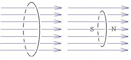
Suppose that we place a bar magnet along the axis of a circular loop
of
wire with the north pole nearest to the loop.
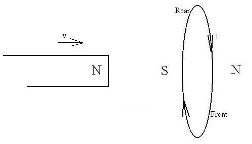
Now, we'll nudge the magnet ever so gently toward the loop. As
a result, the flux through the loop changes and a current is
induced.
We saw in the last
section that a current loop produces a magnetic field of its own
which
resembles that of a bar magnet. Let's assume that the current
flows
so that that a south pole is formed on the side of the loop nearer to
the
magnet. This south pole will attract the north pole of the
magnet,
accelerating it toward the loop. As a result, the flux through
the
loop will change at an even faster rate, which increases the emf,
and therefor the curent, in the loop, making the south pole even
stronger.
This increases the force on the magnets, which accelerates even more
quickly,
which... well, you get the point. The end result is that we get a
very quickly moving and energetic piece of iron, while only having put
in a very tiny amount of energy. Now, one might ask a particular
question at this point:
If that were so, we would expect the initial tap to have been
unnecessary;
the magnet would have started moving all on its own.
So, clearly, this choice of current flow is incorrect, and the only
other choice must be the correct one.
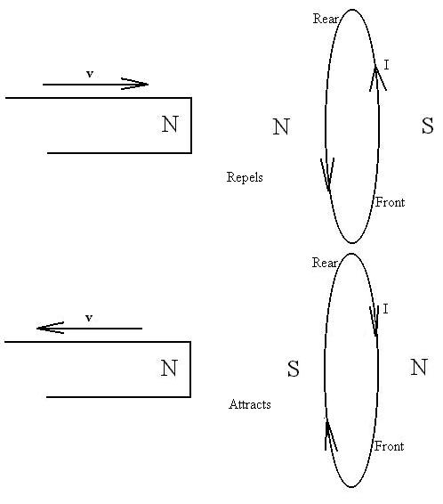
We can think of the situation this way: the direction of the induced
current is always in such a way as to oppose whatever you try to
do.
If you try to bring a south pole toward the loop, the current will flow
such that a south pole will form on the side near the magnet's south
pole,
thus attempting to push the magnet away. If you try to pull a
north
pole away from the loop, a south pole will form on that side to attempt
to pull it back again.
Try an example. Suppose that a loop of wire is lying
horizontally
on the table before you, and that you are bringing a bar magnet down
toward
it, south pole first. In which direction wil the induced current
flow?
So, in general, as the magnetic field though a loop gets weaker,
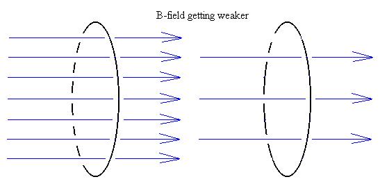
the emf will be the same as it would be for a magnet being pulled away
from the loop:
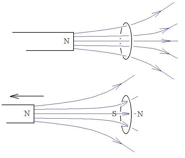
What would we do if the flux were changing due to a change in the area
or the orientation of the loop?
We need to be able to twist the situation around a bit until it looks
like a magnet moving towards or away from the loop. In that case, fewer
B-field lines will be passing through the loop to the right, which we
can
once again simulate by pulling the magnet shown above away to the left.
Then, we know that the current induced in the loop will try to form a
south
pole on the left side of the loop, and so the current must be going
down
the front side and up the back side of the loop.
Similarly, if we were to tilt the loop, so that fewer B-field lines
pass through it, we could simulate that situation also with a north
pole
on the left being pulled away.
This last concept, that the induced emf will try to act to oppose
any
change in the system is called Lenz's Law; we'll remind
ourselves
of it by inserting a negative sign in the relationship developed above,
which then appears as
e = (-) N dfM/dt.
This is known as Faraday's Law of Induction.
Faraday's Law does not come out of thin air; we can show that it is
equivalent to an effect we've seen before. Consider the very
special
case of a U-shaped wire situated with its plane perpendicular to a
uniform
magnetic field, B. Consider further a light, conductive bar of
length
l,
the ends of which lie on the wire and which is constrained to move
along
the wires without friction, as shown.
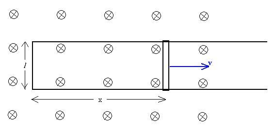
Let's assume that the bar is distance x from the left end and that
it is moving to the right with speed v. If we look at the loop
formed
by the bar and the three sides of the wire to the bar's left, we see
that
there is a magnetic flux given by
FM = BAcosqB,A
= B*(lx)*1.
Faraday's Law then indicates that (since N = 1 here)
e = (-)
N dFM/dt
= (-) d(Blx)/dt
= (-) Bl d(x)/dt
= (-) Blv.
The direction of the emf can be obtained this way: Increasing
the area of the loop increases the flux in that same way that
increasing
the B-field strength would, and we could do that by bringing
the
north pole of a bar magnet down toward the loop from above the page. Per
the discussion above, this would make an induced north pole form just
above
the loop, and by the RHR, this pole would be formed at that location by
a counter-clockwise current.
Now, instead consider the charges residing in the bar. These
are
moving through a magnetic field with a speed v, and like all such
charges,
they will experience a deflecting force given by
FM = qvB sinqv,B (RHR)
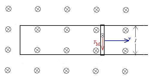
In this case, the angle is 90o, and the electrons wil be
deflected toward the bottom of the page, while protons will be
deflected
toward the top of the page. Since protons are almost 2000 times
as
heavy as electrons, and because they are connected together by atomic
bonds,
and because there may well be other outside forces acting on the bulk
of
this bar which will cancel the magnetic forces on the protons, we shall
ignore said forces and concentrate on the forces on the
electrons.
The force on charge q's worth of electrons will be
FM = qvB.
As the electrons work their way from the top of the bar to the bottom,
work will be done:
W = Fd cosqF,d = FMl
= qvBl.
Since the kinetic energy of the electrons doesn't change (drift
velocity
is constant), this work can be considered to be an increase in
potential
energy:
W = DPE (note that there's no negative
sign,
because the potential energy we're considering is not associated with
the
magnetic force).
What is the emf? It's the difference in potential between the two ends
of the bar, and potential is the potential energy per unit charge:
e = DV
= DPE/q = W/q = qvBl/q = Blv.
What's the direction of this emf? We said that the electrons
will experience a force toward the bottom of the page, which means that
the current is actually flowing toward the top of the page in the bar (i.e.,
counter-clockwise around the loop), and so the emf is directed in the
same
manner. Quelle surprise, eh?
The point of this is to demonstrate (for a very easy case, anyway)
that
the emf which seems to appear by magic in a coil is actually due to
real
forces acting on real charges moving though real (or at least, they are
real in our present model) magnetic fields.
In fact, this emf will exist in the bar whether there is a loop
connected
to it or not. In that case, the charges feel the magnetic force,
same as before, but they can not escape around the loop, so instead,
they
will collect at the ends of the bar (one end positive and the other
negative).
As a result, an internal electric field will be set up, runnng in this
case from the top end to the bottom end. Equilibrium wil be
reached
when the electric force on a charge is balanced by the magnetic force:
qE = qvB,
E = vB.
There is a potential difference associated with the electric field
(here, d = l):
e = DV
= (-) Ed = E l = [Bv] l = Bvl,
as before.
Just for fun, let's add a resistor to the circuit and investigate
what
happens to the energy in the system. We've already decided that
there
is an emf in the loop, which will drive a current:
I = e/R = Blv/R.
The power dissipated in the resisor will be
P = I2R = B2l2v2/R.
Where does this energy originate? Since there is a current in
the bar, there is also a magnetic force acting (by the RHR) to the left
of magnitude IlB. There may well be magnetic forces on the
other parts of the loop, but since the loop is presumably nailed down,
those forces will be cancelled by mechanical forces. This
magnetic
force should act to slow and eventually stop the bar's motion towards
the
right. To keep the bar moving at a constant speed, as was
stipulated
at the top of this section, we need to apply our own force of
magnitude
IlB to the right.
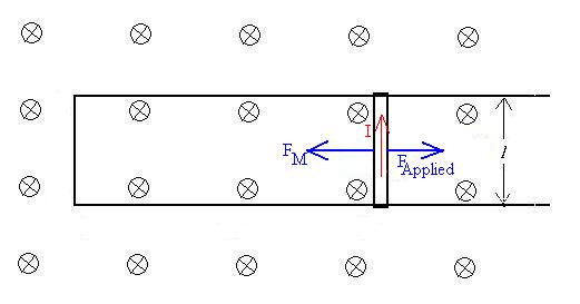
FApplied = IlB = [Blv/R]lB
= B2l2v/R.
Correspondingly, what power must be applied?
P = Fv = [B2l2v/R]v = B2l2v2/R.
So, we see that the energy must come form somewhere, either through
an external agency doing work or perhaps from the kinetic energy of the
bar as it slows.
Self Inductance
Consider a single loop of wire carrying a current, I. The loop
produces
a magnetic field which passes through itself, causing a magnetic flux
over
the area of the loop; this flux will be difficcult to calculate, since
it involves a number of geometric effects, but certainly, we can lump
all
of these effects together and say that the flux is proportional to the
current with a constant we'll label L: FM
~
LI. If the current I were to change (for whatever reason), then
there
would be an emf induced in the loop:
e = (-)dFM/Dt=
(-)
LdI/Dt;
we will call L the self-inductance of the coil. If there
were more turns to the coil, we'd have a similar result with more
constant
terms lumped into 'L.' The unit of self-inductance is the henry
(H). The minus sign representing Lenz's Law reminds us that the
induced
emf in the coil will act to maintain the present state of the system;
for
example, if the current tries to increase, the induced emf will
be directed so as to oppose that increase.
Let's examine a system for which it might be fairly easy to
calculate
L: the solenoid. Consider a solenoid of N turns with length l
and radius r. If l >>r, we might think that the
B-field
generated
inside the solenoid is approximately the same as that in an infinite
solenoid:
B = monI = mo[N/l]
I.
Each loop of the solenoid will experience a magnetic flux; since the
magnitude of the B-field is constant all along the cross-sectional area
and everywhere perpendicular to the cross-sectional area, the flux is
easy
to calculate:
FM = BA = mo[N/l]
I pr2.
Now, the emf is given by Faraday's Law:
e = (-)
N dFM/dt
= (-) N d[mo[N/l]
I pr2]/dt.
Since the current is the only quantity changing here, this can be
rewritten
as:
e = (-) [moN2pr2/
l
] dI/dt.
Comparison of this result to our expected form reveals that
Lsolenoid = moN2pr2/l.
Applications of inductors include:
power spike and noise suppression (the rapidly changing currents
associated
with the spikes create a reverse emf in the inductor), high frequency
filtres
(same effect), and automobile ignition systems (rapidly disconnecting
an
inductor from a 12.6V driven current can produce a several thousand
volt
emf across the spark plug gap).
Mutual Inductance
We can also talk about the mutual inductance (M) of two coils
not
actually in electrical contact with one another. Using an
argument
similar to the one above for self-inductance, we can write that:
e1 = (-)
M12 dI2/dt
+ (-)L1 dI1/dt,
e2 = (-)
M21 dI1/dt
+ (-)L2 dI2/dt.
Here is a useful example of mutual inductance. Consider two
coils
with N1 and N2 turns, respectively, each wrapped
around a frame made of soft iron, which is easily magnetized.
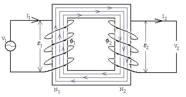
We'll drive a current through coil 1 with a varying voltage,
V1. Since V1 is varying in time, the
current
I1 will do so also. I1 causes a magnetic
field
in coil 1, some of the lines of which pass through coil 2. Now,
the
soft iron has the property of re-directing these magnetic field lines
through
itself, so that a very large fraction of them will pass through coil 2;
in fact, we'll assume that 100% of them do so, although in real life,
the
figure is more like 96%. Now, when I1 changes, the
flux
through coil 2 will induce an emf, perhaps causing a current I2
in coil 2, which will in turn cause its own magnetic field which also
passes
through both coils and is changing with time (although, the existence
of
I2 is not necessary to this derivation). At any rate,
each
loop in each of the two coil experiences a flux due to the fields
generated
by itself and by the other loops. These fluxes are the same
(regardless
of their sources), since one interpretation of the flux is that it is
proportional
to the number of B-field lines passing through, and we stipulated that
all lines pass through each coil. So,
FM1 = FM2.
Now, if two quantities are always equal, then their time rates of
change
must also always be equal, so,
dFM1/dt
= dFM2/dt.
Now, each coil will have an induced emf described by Faraday's
Law:
e1 = (-)
N1dFM1/dt
e2 = (-)
N2dFM2/dt.
and so
e1/N1
=
(-)dFM1/dt
= (-)dFM2/dt
= e2/N2
e1/N1
=
e2/N2
By Kirchhoff's Loop Law, V1 + e1
=0 and V2 + e,
=0, so
V1/V2 = N1/N2.
So, we see that we can use such a device (called a transformer)
to step-up or step-down the amplitude of a time varying voltage.
We did a demonstration with a transformer with a turn ratio of
10:1.
By applying a 10V sinusoidal voltage to the primary coil, we
could
obtain a 1 volt output across the secondary coil, or, by
reversing
the coils, a 100 volt output.
You may see transformers every day. The power company produces
electricity at about 1000V, then steps it up to 100,000V for
transmission
over long distances (thousands of miles). As the lines get closer
to the consumer, other transformers lower the voltage back down to the
thousands, then to the hundreds. Normally, each house has a
transformer
just outside (either on a pole or often just sitting on the front lawn)
which lowers the voltage to 220V. Why not lower it right away to
the familiar 110V?
Typically,
electric ranges and air conditioners run on 220V.
RC Circuits
Consider a battery, resistor, and capacitor arranged in a series
circuit,
along with a switch which will allow us to connect and disconnect the
battery
easily while maintining the continuity of the circuit.
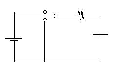
What will be the behaviour of the current in the circuit as a function
of time after closing the switch so that the battery is in the
circuit?
Let's specify that we will start with the capacitor uncharged.
Write
Kirchhoff's Loop Law, assuming that the current is positive in the
clockwise
direction:
IR = eB
- VC
IR = eB
- q/C.
Unfortunately, we have two variables here, the charge q and the current
I. We need another relationship to have enough information to
solve.
Can you think of a relationship between I and q?
So, I = dq/dt, and we obtain
R[dq/dt] + (1/C)q = eB.
Such an equation, which contains a quantity and some rate of change
of that quantity, is called a differential equation.
First,
we need to find the homogeneous solution, qH, found
when the right
hand side is set to zero:
R[dq/dt] + (1/C)q = 0.
Re-arrange to obtain
dq/q = -[1/RC] dt.
Integrate:
ln q = -t/RC + A, where A is a constant of integration.
Exponentiate:
qH = A' e- t/RC, where A' = eA is
a new constant.
Now, we look for a particular solution to take care of the
right-hand
side, eB.
We might well guess that
qP = eBC,
since substitution of this guess into the original equation gives:
R[0] +(1/C)[eBC]
= eB.
So, the general solution is
qG = qH + qP = A' e- t/RC
+ eBC.
To find A', we look at the initial conditions. In our
example, we said that q = 0 at t = 0, so substitute this information
into the
solution to obtain
0 = A' e- 0 + eBC.
A'= - eBC.
So the complete solution for this inital condition is
q(t) = eBC
(1 - e- t/RC).
The current in the circuit is given by
I = dq/dt = [eB/R]e-
t/RC.
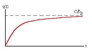
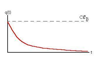
Now, let's let the circuit run for a very long time, so that the
capacitor
charges up as much as it can. In the end, the voltage across it
will
be the same as eB
and the charge will be
qt=oo = eBC.
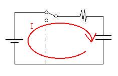
Flip the switch over to the other position, so that the battery is
no longer in the circuit. The capacitor will of course begin to
discharge
through the resistor (we'll expect the current to to be negative here).
Let's write Kirchhoff's Loop Law again:
R[dq/dt] + (1/C)q = 0.
We already know the solution to this equation:
q(t) = A' e- t/RC,
and, since the capacitor starts off with a charge of eBC,
we see that A' = eBC,
so,
q(t) = eBC
e- t/RC.
The current is given by I = dq/dt = - [eB/R]e-
t/RC.
What if the capacitor had not fully charged up? Then, instead
of eB
as the initial voltage, we'd just use Vo (= qo/C).
The quantity RC is often referred to as the capacitive time
constant
of the circuit,
tC = RC,
which can be thought of as the time necessary for some quantity to
decay to 1/e of its initial value. Conceptually, it is similar to
the notion of a half-life, except that is the time necessary to
fall to 1/2 of the initial value.
So, we could write that
q(t) = eBC
(1 - e- t/tC);
I(t) = [eB/R]e-
t/tC
(Charging from empty case)
q(t) = eBC
e- t/tC;
I(t) = - [eB/R]e-
t/tC
(Discharging from full case).
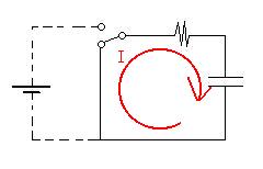
LR Circuits
In a similar way, let's consider a series arrangement of a battery,
resistor,
and inductor.
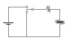
Let's close the switch, so that the battery is in the circuit, at time
t=0:
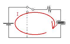
Kirchhoff's Loop Law states that
IR = eB
+ eL
IR = eB
- L dI/dt.
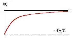
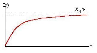
Once again, we have a differential equation, the solution of which
is (if we assume that the current is initially zero):
I(t) = [eB/R](1
- e- tR/L).
If we wait for a very long time, the current will achieve an
ultimate
value of
IFinal = eB/R.
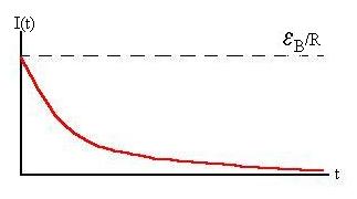
At that time, let's quickly switch the circuit to remove the battery.
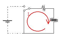
Since the inductor will oppose the drop in the current, it will work
to keep the current flowing. Kirchhoff's Loop Law in that case
is:
IR = - L ddI/dt,
the solution to which is
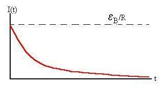
I(t) = [eB/R]e-
tR/L.
Here, we can define the inductive time constant tL
as L/R, so that these equations become:
I(t) = [eB/R](1
- e- t/tL),
and
I(t) = [eB/R]e-
t/tL.
Consider this. In each of the cases discussed above, the RC
and
the LR circuits, current flowed even after the battery was
disconnected,
even if it decreased pretty rapidly towards zero. Since there was
current flowing through a resistor, we know that energy was being
dissipated as heat. From where did this energy come if not from
the
battery? We'll, in the case of the RC circuit, we've already
discussed
how energy can be stored in a capacitor:
UC = 1/2 [1/C] Q2.
So, we might surmise that energy had to have been stored in the
inductor
as well. We will assert now (and show later) that the energy
stored
in the magnetic field in an inductor is
UL = 1/2 L I2.
Continue to the Next
Section
of Notes
Return to the Notes Index
D. Baum 2001