Section 2-5 - Magnetism: Effects & Causes
The Magnetic Field
Gauss's Law for Magnetism
Interactions
between
Currents
and Magnetic Fields
Biot-Savart Law
Ampere's Law
Magnetic Moment
Causes of Magnetic
Effects
in Materials
The Magnetic Field
Magnetism is an effect which has been known for several
millennia.
It was found that pieces of a certain kind of rock, called lodestone
(Fe3O4),
can attract and/or repel one another, as well as other bits of
metals.
These rocks were common in a province near Turkey named Magnesia, and
so
the effect is called magnetism. When suspended and
allowed
to rotate freely, these rocks always orient themselves the same way;
the
end which points toward the north is called a north-seeking-pole (or
just
north
pole), and the other end is the south-seeking-pole (south
pole).
This allows the construction of which important navigation
tool?
We find that magnetic poles always come in pairs, unlike electric
charges;
whenever one type of pole is present, the other type must be somewhere
near. There is a theory which postulates the existence of a magnetic
monopole, but none has been seen to date.
We can make artificial lodestones from iron (and other materials),
which
we call magnets. Investigating the interactions between
magnets,
we find that:
Like poles repel,
Unlike poles attract.
In order for a compass to work, what must be at (or near) the
earth's
Geographic North Pole?
This is very similar to the rules that govern the interactions
of
electric
charges, so perhaps some analogies can be drawn.
For example, can we model the interactions of two poles with a magnetic
field, somewhat similar to the electric field? Since there
are
no magnetic monopoles to use as magnetic test charges, we will instead
use magnetic dipoles as our test objects. We saw in a previous
section
that electric
dipoles will tend to align with the electric field. Let's
place
some small test compasses in the vicinity of a larger magnet:
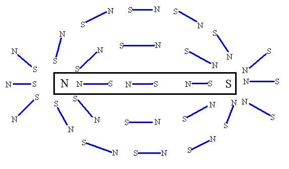
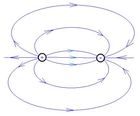
It seems that we could indeed think of the magnetic dipoles as aligning
with a magnetic field, which resembles fairly closely the electric
field
for two equal but opposite charges:
So let's define the magnetic induction field (symbol B,
unit the Tesla; see Note,
below) and arbitrarily choose its direction as
follows:
consider the test dipoles to be little arrows with the point at the
north
end that point in the direction of the magnetic field:
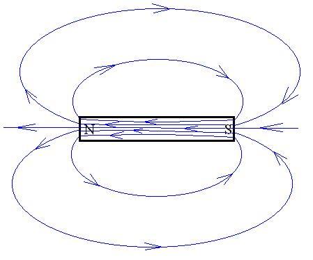
We see that the field runs from the north pole to the south pole, except
inside the magnet, where it runs from south pole to north pole.
This
is somewhat different from the situation with charges, in which the
electric
field ran from positive charges to negative charges. Here, we see
that the magnetic field lines instead form closed loops.
Gauss's Law for Magnetism
We defined the electric flux through a surface to be
FE =  Eperp dA.
That is, we look at each little piece of surface area dA
and multiply that area by the perpendicular component of the electric
field
at that point, counting the product as positive if the field points
from the inside to the outside of the surface, and negative
otherwise. We found that, if we sum this quantity up over a
closed
surface, that the the result is proportional to the charge enclosed by
the surface:
FE =  Eperp
dA
= 4pkeqenclosed.
Eperp
dA
= 4pkeqenclosed.
Perhaps there is a similar relationship for the magnetic field.
We define the magnetic flux (unit, the Weber) through a closed
surface as:
FM = Bperp dA
Consider a closed surface and calculate the total magnetic flux through
it. As for the electric flux, let FM
be positive if the field points from the inside to the outside of the
surface, and negative if it points from the outside to the
inside. Remember that an alternate picture of the electric flux
was
the
net number of electric field lines that pass through the
surface.
What, then, is the total magnetic flux through a closed surface equal
to?
This result will be correct so long as there really is no such thing
as a magnetic monopole.
Interactions
between
Currents
and
Magnetic Fields
We performed a demonstration. We used a horseshoe magnet to
produce
a magetic field in the vicinity of a current carrying wire, and saw
that
a force was exerted on the wire. We saw that the magnitude of the
force depended on the size of the current, the strength of the field,
and
the length of the wire. If we had done very careful quantitative
measurements, we would have seen that:
FM ~ B
FM ~ I
FM ~ L.
In addition, we saw that the force was directed at right angles to
the direction of the current and to the direction of the B-field.
We suspected that we might be able to predict the direction of the
force
using the Right-Hand-Rule (RHR), if we take the current direction as
the
first vector and the field direction as the second. If true,
there
should be a dependence on the relative orientation of the current and
the
field, and this could be found to be true by doing careful quantitative
measurements. So,
FM= ILBsinqI,B (RHR),
or F = L I x B.
That is, point your forefinger in the direction of the current, your
middle finger in the direction of the B-field, and your thumb should be
in the direction of the force.
Now consider the effects of a magnetic field on individual charged
particles.
A cathode ray tube (CRT) such as those in televisions shoot a
stream
of electrons toward a screen, which is covered with a fluorescent
material
which glows as the electrons strike. We orient the magnetic field
in different ways in the vicinity of the electrom beam, and find a
similar
deflection. Suppose that the beam is coming out toward you and
that
the magnetic field (from a horseshoe magnet) is pointing toward your
left.
Based on the previous discussion, which way would you expect the force
on the electrons to be directed, as evidenced by the their deflection?
Did you get the wrong answer? Why?
Is there an angle dependence of the force? We tested this by
turning the magnet around and saw that the deflection becomes smaller
as
the B-field becomes more parallel (or anti-parallel) to the velocity.
Let's guess a relationship for the force:
We expect that the force is proportional to the charge on the
particles:
F ~ q. This could be verified by using alpha particles instead of
electrons
or protons.
We could vary the speed of the particles, ands we would find that F
~ v.
We can add magnets to vary B, and we find that F ~ B.
Also, the angular dependence F~ sinqv,B,
so
that
FM = qvB sinqv,B
(RHR), or F = qv x
B
Note: Some define the magnetic field line as that path along which a
charged particle can move and experience no magnetic force.
Is this consistent with our previous result? In a naive way,
we
can write that, for a wire,
FM = ILBsinqI,B (RHR)
= [q/t]LB sinqI,B (RHR) = q[L/t]B
sinqI,B (RHR) = qvB sinqI,B
(RHR) = qvB sinqv,B (RHR)
or F = qv x B.
where we understand that the direction of the product of q and v is
in the direction of the current (that is, if q is positive, v and I and
parallel, but if q is negative, then qv and I are parallel).
Let's consider a special case of a charged particle (mass m
and
charge +q) entering a region of uniform magnetic field (B) so
that
initially, v and B are perpendicular.
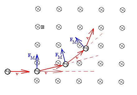
There will be a magnetic force acting on the particle, FM
= qvB (remember that we stipulated that qv,B
is 90o). This force will be direcred as shown, and
will
deflect the path of the particle from its original direction to the one
shown. Once it has arrived at its 'new position' with its new
velocity,
there will still be a magnetic force, but that force will be directed
at
a slightly different angle, as shown. This causes another
deflection
and the particle moves to the third position shown, et c.
What can we say about the speed of the particle?
Keeping in mind that this process is much smoother, and that the path
taken is not really polygonal, can we guess what shape trajectory the
particle
will take?
What kind of force is required to keep an object moving in such a
trajectory?
What provides that force in this situation?
So, we have that
FM = FC
qvB = mv2/r
qB = mv/r
r = mv/qB.
Let's look at this same situation in a slightly different way to
obtain
an interesting result:
FM = FC
qvB = mrw2
qrwB = mrw2
qB = mw
w = qB/m.
That is, the angular velocity (or, more interestingly and equivalently,
the frequency) of a charged particle in a magnetic field is independent
of the energy (speed) of the particle!
This result is the foundation for several interesting devices,
notably
the mass spectrometer. Suppose that we wish to identify a
material from its molecular mass. We place the material in an
oven
which vaporizes it and spews it out at high speed. Unfortunately,
there is a distribution of speeds (the Maxwell distribution). After
passing
through various collimators to produce a well defined beam of
particles,
they molecules are directed through an electron stripper, which
removes one (or more) electrons. The now charged particles travel
through a velocity selector, which is a region of crossed
electric
and magnetic fields.
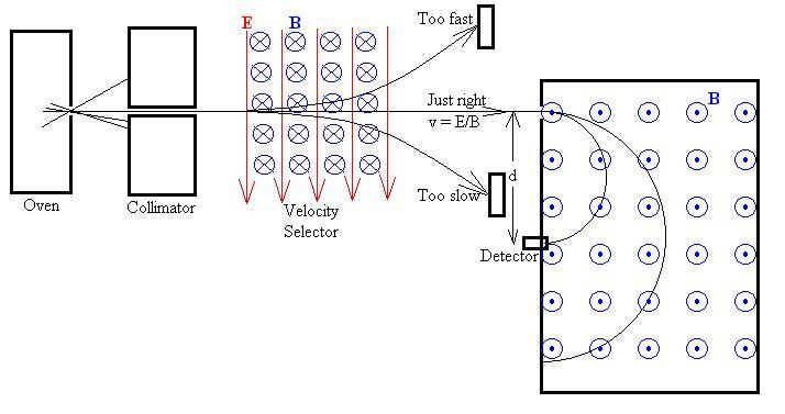
There is an electric force qE on the particle toward the bottom of
the page and a magnetic force qvB directed toward the top of the page
(check
it!). The electric force is the same regardless of the speed of
the
particle, but the magnetic force is proportional to the speed of the
particles.
For fast particles, FM is greater than FE, and
the
particles will be deflected upward. For slow particles, FE
is greater than FM, and the particles are deflected
downward.
However, for particles with just the right speed, the forces cancel and
the particles travel in a straight line. This will occur when
FE = FM
qE = qvB (assume q is not zero)
E = vB
v = E/B.
Now, the particles enter the main spectrometer, a region of uniform
B-field, and their paths are bent into circular arcs as shown.
Since
all particles now have the same speed, and (we hope) the same charge,
and
they are experiencing the same B, we find that the radius of each orbit
is proportional to the mass of the particle:
r = [v/qB] m.
By running a detector along one edge of the chamber and recording the
number of particles arriving as a function of distance d (=2r), a
spectrum
of the masses of the particles can be taken and the materials
identified.
m = [qBSPECTBSELECT/2ESELECT]d.
Often there are complications: for example, some particles will be
doubly or triply charged, giving rise to extraneous lines at m/2 and
m/3,
and the molecules are often broken into fragments which also register
as
peaks in the spectrum.
This process was initially used to separate uranium early in the
wartime
effort to construct the atomic bomb. There are several isotopes
of
uranium, the most common being U-235 and U-238. U-235 is useful
for
bombs, while U-238 is useful in power reactors, but will squelch the
necessary
fast chain reaction in a bomb. They can not be separated
chemically,
since they have the same electronic structure. A method was
developed
to use the mass spectrometer to separate the isotopes, but the
production
rate was eventually deemed to be too slow.
Consider these questions:
What shape path will a charged particle take when injected into a
uniform
electric field with its initial velocity not perpendicular to the
field?
What shape path will a charged particle take when injected into a
uniform
magnetic field with its initial velocity not perpendicular to the
field?
Biot-Savart Law
We have seen that magnetic field can have an effect on electric
currents.
Now we shall discuss the observation that currents can cause magnetic
fields.
Previously, we had assumed that these fields were caused by special
rocks
(which we can produce artificially, it's true). Later, we will
present
a naive model to reconcile these two sources of B-field. How do
we
know that currents cause B-fields? Weirdly enough, it is from a
lecture
demonstration gone bad. Oersted had wanted to show that currents
in wires do not affect compass needles, but he learned the hard way
that
they do, as the compass swung around in front of his audience.
We won't attempt to justify the following result in anyway, other that
to say that it is based on careful experimentation and
observation.
Consider a current of arbitrary shape; we wish to find the magnetic
field
caused by this current at point P.
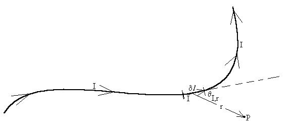
Consider a short piece of the current of length dli,
which produces a contribution dBi
to the field at point P. We find that the magnitude of dBi
is given by
dB = kM
I dl
sinqI,r /r2,
where kM is a constant to make the units work out right
(kM = 10-7 Tm/A, exactly), r is the
distance
from the current element and the point P at which we are finding the
field,
and qI,r is the angle between
the
direction of the current and the direction to the point P. We
find
that the direction of this contribution to the B-field is given by a
Right-Hand-Rule:
the index finger points in the direction of the current, the middle
finger
points toward the point at which the field is being found, and the
thumb
points in the direction of dB.
In
this example, the contribution from the curremt element shown is
into
the page.
To find the total field at P, we need to add up all the contributions
from each little piece of the current, keeping in mind that this must
be
vector
addition. Also, ri and qI,r
may well be different for each current element:
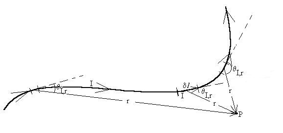
Even then, that only gets the B-field at one spot; the calculation
must be repeated for any other spot. In some special cases, we
may
find that the contributions all point in the same direction, in which
case
the vector addition simplifies to algebraic addition.
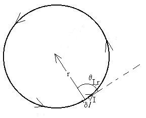
Example:
Find the B-field (magnitude and direction) at the centre of a circular
loop of radius R carrying current I as shown.
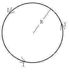
Consider a short bit of the loop of length dli.
The
distance
r from this piece of current to the point at
which
we are finding the B-field is R, and the angle between the current
direction
and the direction to the centre is 90o. From the
Right-Hand-Rule,
the field this piece of current causes points out of the page.
What's more, all these things are true for any of the current
elements. So, the vector sum we must do reduces to an algebraic
sum:
B =  dB = kM
I dl
(sinqI,r
)
/r
2,
dB = kM
I dl
(sinqI,r
)
/r
2,
But we said that the current is the same in each element, r = R for
each element, and q is 90o (so
sinq
= 1) for each element, so we can factor these constants out of the
integral:
B = [kM
I /R 2] dl
.
The sum all around the loop of all the small lengths is the
circumference
of the circle, 2pR, so,
B = [kM
I /R 2] 2pR
= 2pkM I /R.
Now, we will make a change of the constant, just as we changed 4pke
into 1/eo. We let mo
= 4pkM, so that the result
becomes
Bcentre = mo I/2R.
Consider this current arrangement:
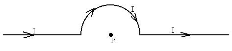
The straight portions of the wire extend out to infinity and the curved
jag is a semi-circle of radius R. Find the magnetic field at P.
Here is another example:
Infinitely long, straight wire with current I
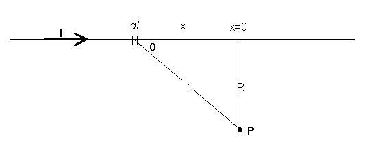
Consider the P point shown. The small length of wire dl will produce a contribution to
the magnetic field at P
dB = kM
I dl
sinqI,r /r2
To change variables for integration, let r = [R2 + x2]1/2,
dl = dx, and sinq
= R/r = R/[R2 + x2]1/2.
dB = kM
I dx
R
[R2 + x2] -3/2
Since each contribution dB
will, by the RHR, point into the page, the total field at P is the
simple sum of all the contributions (the magnitude of the sum is the
sum of the magnitudes):
BP = -INF+INF
kM I dx
R
[R2 + x2] -3/2 = kM I Rdx [R2
+ x2] -3/2 = kM I R [x/R2[R2
+ x2] 1/2 -INF|+INF]
= 2kM I /R = mo I/2pR.
Ampère's Law
Ampère's Law can be shown to be identical to the Biot-Savart Law
(we
won't
do so). From an operational point of view, Ampère's law is
to
magnetism
what Gauss's law is for electricity; for sufficiently nice symmetries,
we can use it to determine the magnetic field caused by current
distributions.
Suppose that we have a current which is producing a magnetic field
B.
Let's draw an imaginary closed loop in space in the vicinity of the
current.
Break the loop up into many very short lengths, dl.
As
we
follow the path along the loop, we look at the component of the
magnetic
field which is parallel (or anti-parallel) to the loop and multiply it
by the length of the little bit of the loop:
B|| dl.
This is analogous to choosing an imaginary surface and looking at the
perpendicular component of the electric field in Gauss's law:
Eperp dA
Now, let's add up all these terms all the way around the loop; if the
B-field component is in the same direction in which we are traversing
the
loop, we'll call the term positive and if the component is opposite to
the direction we are going, we'll call it negative. This is again
analogous to calling the flux positive if the E-field points from the
inside
of the gaussian surface to the outside, and calling it negative if the
E-field points from the outside in. When the sum is complete, the
result will be proportional to the net current passing through the
loop:
 B||
dl
= mo Ienclosed
B||
dl
= mo Ienclosed
or more explicitly mathematically:
B .dl
= mo Ienclosed
Just as for Gauss's Law, this is always true, but it may be useful
for finding B only in certain symmetric situations. In Section
2-1, we tried to find surfaces for which either the E-field was
along
the surface (so that Eperp = 0) or if not so, then exactly
perpendicular
and constant in magnitude. Similar hopes and dreams run wild
here:
we'd like to choose loop paths such that either B is perpendicular to
the
path (and so there is no contribution to the sum) or if not, then
preferably
along the path and constant in magnitude.
Consider the example of an infinite, straight, current-carrying
wire.
First, we need to at least consider the Biot-Savart Law (and the RHR)
to
get an idea of what the B-field looks like:
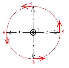
It seems clear that the B-field will form circular loops around the
wire, as shown. Furthermore, symmetry arguments can be made that
the magnitude of the field at points at any given distance r from the
wire
will be the same. It seems that a good choice for our imaginary
loop
might be a circle of radius r which lies along one of the field
loops.
In that case, we write that
B||
dl
= mo Ienclosed
Since B is parallel to the loop at all points, we can replace B||
with
plain ole B:
B dl
= mo Ienclosed
Also, since we argued that the magnitude of B is the same everywhere
on the loop, we can pull it out of the integral:
Bdl
= mo Ienclosed
The integral has been reduced to the length of the loop, i.e.,
the
circumference of the circle:
B 2pr = mo
Ienclosed.
B = [mo Ienclosed]/2pr,
and in this case, Ienclosed is just the given current I,
so
B = mo I/2pr.
It's acceptable to have r in the answer since r corresponds to the
real distance from the wire at which we want to find the field.
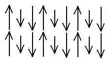
Consider the infinitely
long
solenoid,
which is a wire coiled up along a cylindrical form, somewhat like a
'slinky.'
Let's draw this schematically by slicing the solenoid in half along its
length:
The lower vectors represent the current coming under the bottom of
the solenoid, while the upper vectors represent the current rolling
back
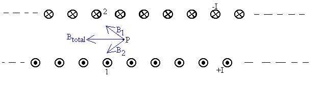
over the top of the solenoid. We pick a point P inside the
solenoid
on its central axis at which to find the field. Consider one
little
bit of the current, here labeled '1.' The B-field from that bit
of
current is in the direction shown and is labeled B1.
Likewise
for a bit of current exactly opposite it and the same distance from
point
P, labeled '2.' We see that the net field is directed to the
left,
since the vertical components will cancel. This will be true for
all such pairs we pick, so the net field is to the left. Also, we
can say that the magnitude of B will be the same all along that central
axis, since the solenoid is infinite in length and we can shift it to
the
right or left any amount and the system should appear to be the
same.
This is true if the points we look at are on the central axis of the
solenoid;
what if we look at a point off axis? We shall contend that the
B-field
is to the left everywhere inside the solenoid, based again on symmetry
arguments.
What about the field outside of the solenoid? We contend that
the B-field there is to the right and very weak, weak enough to
neglect.
Remember that B-field lines from closed loops, so the lines running
inside
the solenoid towards the left end have to loop back on the outside to
the
right end. Since the solenoid is infinitely long, we might expect
that the lines are very spread out from each other on the 'return
trip,'
and since the strength of the field is related to how closely the lines
are spaced, we can say that the field is very weak.
Let's choose a rectangular path of length L along which to calculate
our sum:
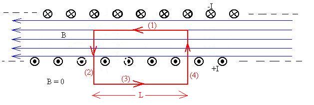
Label the segments of the path as shown. The sum can be written
as:
B dl
= mo Ienclosed
= (1) B||
dl
+(2) B||
dl
+ (3) B||
dl
+ (4) B||
dl
= mo
Ienclosed.
Along (1), B is parallel to the path and has constant magnitude, so B||
= B, and so it can be factored out of the integral to give B (1) dl
= BL.
Along (2), B is either zero or it is perpendicular to the path, so
the contribution is zero.
Along (3), B is zero, so the contribution is zero.
Along (4), B is either zero or it is perpendicular to the path, so
the contribution is zero.
So, we're left with
BL = mo Ienclosed.
Now, work on the right hand side of the relationship. Ienclosed
depends on how many turns of the solenoid are enclosed; let's just say
N turns. Then,
BL = moNI.
B = moNI/L.
Now, we have a problem. When we discussed Gauss's Law, we pointed
out that there should be no quantities in our final answer that are
dependent
on the dimensions of our imaginary surface. In this result, we
have
two quantities that depend on the size of our imaginary loop, namely
the length L
and the number of turns enclosed, N. What is the resolution to
this
paradox?
Let n = N/L, so that the result becomes
B = monI.
Now, note that this result does not depend on where we placed
part (1) of the rectangular loop, so that the magnitude of B is the
same
across the cross-sectional area of the solenoid. This means that
solenoids are very useful for producing extremely uniform magnetic
fields,
such as necessary for NMR experiments.
Lastly, let's look at the example of a flat, infinite sheet of
current.
The current at any spot is directed parallel to some given axis (in the
figure, it's all out of the page). Since the total amount of current is
infinite (so long as it's not zero), we should define a current
density,
the amount of current per unit length: J
= I/L. This is not the usual current density J, the
current
per
unit area. Look at some point a distance r from the sheet and try
to determine the appearance of the B-field.
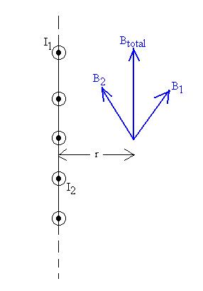
Consider two currents, I1 and I2, each producing
a contribution to the total field; we see that the vertical components
add and the horizontal components cancel. In addition, since we
can
slide the sheet up or down (or for that matter, into or out of the
page)
some distance and it will still look the same, we can say that the
magnitude
of the B-field is the same value at any point a given distance r from
the
sheet. What's more, the field on the other side of the sheet at
distance
r will have that same magnitude, although we can see quickly with the
Right-Hand-Rule
that the direction is reversed.
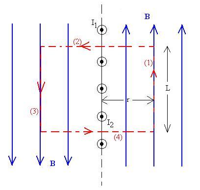
Let's choose a rectangularly shaped loop about which to sum.
Since we as yet have no idea how the B-field strength varies with
distance
from the sheet, we'll draw the loop symmetrically as shown; then at
least
the field magnitudes along parts (1) and (3) will be the same.
So,
B||
dl
= mo Ienclosed
= (1) B||
dl
+(2) B||
dl
+ (3) B||
dl
+ (4) B||
dl
= mo
Ienclosed.
Along (1), B is parallel to the path and has constant magnitude, so B||
= B and it can be factored out of
the integral to give B (1) dl
= BL.
Along (2), B is perpendicular to the path, so the contribution to the
sum is zero.
Along (3), B is parallel to the path and has constant magnitude, so B||
= B and it can be factored out of
the
integral to give B (3) dl
= BL.
Along (4), B is perpendicular to the path, so the contribution to the
sum is zero.
So, we're left with
2BL = mo Ienclosed.
Now, work on the right hand side of the relationship.
Ienclosed
= J L, so
2BL = moJ
L.
B = moJ/2.
Note that the answer is independent of r, the distance from the sheet.
Magnetic Moment
Consider a loop of wire carrying a current I (since this is a three
dimensional
situation, we'll label the front and rear parts of the loop):
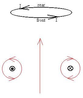
In the lower half of the figure, we've sliced the loop in half with
a plane parallel to that of this page, so that only the two bits
passing
through that plane are now shown. Let's get an idea of what the
B-field
produced by this loop of current looks like. We previously used
the
Biot-Savart Law to show that the field points along the axis of the
loop points
as shown, and when we are near the wire, we can consider the portion
nearest
us to behave much like a straight bit and ignore the more distant bits,
thus producing the field as shown here. Let's also fill in the
field
imaginatively in the other regions, keeping in mind that there is
probably
a smooth transition from one region to the other:
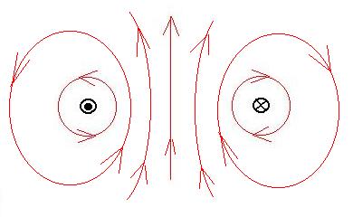
Now, does this field arrangement remind us of anything? Perhaps
the magnetic field caused by a bar magnet?
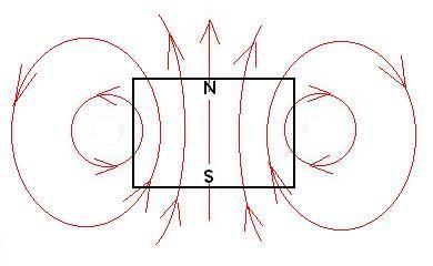
So, we should expect a loop of current to behave like a bar magnet
or compass needle, and we should be able to predict which side of the
loop
will act like a north pole (short-hand Right-Hand-Rule: Curl fingers of
RH in direction of the current, and the thumb will be where the north
pole
is). We did a quick demonstration of this and saw that, indeed,
the
current loop was attracted and repelled by a bar magnet as expected.
Why does a bar magnet act like a current loop? See below.
Let's consider a rectangular loop (length l and width w)
carrying
current
I, in a uniform magnetid field, B, the plane of which
is inclined to the direction of the field by some angle q,
which we will measure between the magnetic field and a line
perpendicular
to the plane of the loop:
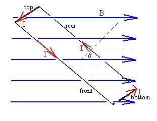
Consider a more schematic view of this loop:
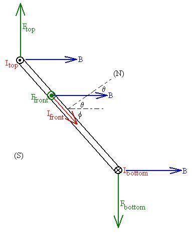
In this figure, the current running up the back leg is not shown.
From the previous discussion, we might well expect that the current
will
cause to form a north pole somewhere up and to the right of the loop
(and
a south pole down and to the left) and that, as a result, the loop will
begin to swing clockwise to align itself with the magnetic field.
Let's examine this in closer detail:
The loop comprises four legs or straight sections, each carrying
current
I, in a magnetic field B. There will therefor be a magnetic force
on each leg,
FM = ILB sinqI,B
(RHR):
Ftop = IwB sin 90o = IwB (up),
Ffront = IlB sinf (out
of the page), f is the complement of
our
original q.
Fbottom = IwB sin 90o = IwB (down),
Frear = IlB sin (180o - f)
= IwB sinf (into page).
Now, the net force on the loop is clearly zero, but what about the
torque?
On the front and rear sides, the net torque will be zero, since, for
every
bit of current on the front side experiencing a magnetic force, there
is
an oppositely directed current bit experiencing a force in the other
direction
which as acting along the same line as the first force. However,
on the top and bottom legs, the forces do not act along the same line,
and so there will be some net torque. Remembering that
t = rF sinqr,F
(RHR),
divining that r is l/2 (since the loop will most likely rotate
about its centre of mass, although in fact this doesn't really matter)
and that qr,F is the same as our
original q,
ttop = [l/2][IwB]
sinq (into
the
page)
tbottom = [l/2][IwB]
sinq (also
into
the
page),
and the total torque is
ttotal = lIwB sinq
(into
the page).
If there had been N turns in the
loop, the torque would have been N times larger, so let's work that
into
the relationship. Also, lw is the area of the loop, and
it
can be shown that the result valid for this specific case is valid for
any flat loop of area A:
ttotal = NIAB sinq
(into
the page).
Now, we will do what we did in a
similar
situation back in Section 1. We will define a new vector, m,
as the magnetic dipole moment; its magnitude will be NIA and
its
direction will be from the centre of the loop toward the 'north pole'
formed
by the current. We see, then, that the theta in our
result
is the angle between B and m,
and so a Right-Hand-Rule seems appropriate. Try B x m;
that points out of the page, so let's make it t
=
m
x B, or,
t = mB sinqm,B
(RHR).
Loops which are not flat can of
course
also have magnetic moments, but they must be calculated a bit more
carefully.
Here is an example:
Consider a circular loop of
radius
R which has been bent at a right angle along a diameter. What is
the magnetic moment of this current distribution?
One last bit of advice: don't confuse the magnetic dipole moment m
with out magnetic constant, mo.
Now, let's look at this a different way: we can consider a
torque
acting to rotate our current loop, thus causing an angular
acceleration,
or we can develop a potential energy function, and consider said PE to
be converted into kinetic energy as the loop swings around. We
will
make use of the result we obtained for the electric
dipole and guess that
PEdipole = - mB cosqm,B.
Careful experimentation confirms that this guess is acceptable.
Causes of Magnetic
Effects
in Materials
Now, we can return to the beginning of this section and make an attempt
to explain the effect which allows some materials to be magnets; this
is
called ferromagnetism, since the largest such effect is seen in
iron (Fe). We saw in the last section that current loops
can
produce magnetic fields which resemble those of bar magnets, and so the
loops are affected by other magnetic fields in the same way that
magnets
are. Consider an electron, a simple model of which is a rotating,
charged sphere (with an as yet unmeasurably tiny radius) orbiting the
nucleus
in much that same way that a planet orbits the sun. The moving
charge
on the electron is similar to charge moving around a loop, and so a
magnetic
field should be produced.
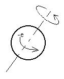
Which end of the electron will act like a north pole?
Let's represent these particles with a little arrow, with the head
of the arrow being the north pole and the tail the south pole.
Think
of it as the electron's magnetic moment. As we progress through
the
periodic table, electrons fill the orbitals, usually quickly pairing as
'spin-up' and 'spin-down' and thus cancelling any net magnetic
moment.
Magnetic effects are seen in materials where there is an unpaired
electron.
This then excludes the noble gases, most even numbered elements, most
ions
(which have either gained or shed electrons to obtain filled outer
shells)
and materials which form co-valent bonds (since electrons from two
atoms
pair up in the bond). The best candidates are elements in the
transition
columns of the table.
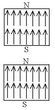
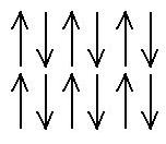
If we were to place two such atoms next to each other, we would expect
them to align in opposite directions, since the north poles would
attract
the south poles, or because this would be the lower energy state:

However, in several materials, the energy considerations are such that
a lower energy state is achieved if the spins align parallel to one
another:

This occurs in only five elements (iron, nickel, cobalt, gadolinium,
and dysprosium), plus a number of alloys. Such materials are said to be
ferromagnetic.
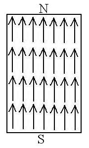
Since this results in an alignment of a majority of these tiny magnets
in the same direction, the result is one big magnet:
Now, of course, in real life, not all will line up, and there are some
fairly easy statistical calculations which can be made for different
conditions.
Consider these questions:
What happens if a magnet gets broken? Do we get a (separate)
north
pole and a south pole?
No, we wouild get two magnets:
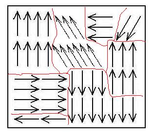
Why are not all pieces of iron magnets?
The magnetic forces causing this ordering are short-range forces,
that
is, the ordering is local only. In most iron, there are regions
called
magnetic
domains in which a majority of the moments are aligned, but the
overall
average magnetization is zero (or close to it).
How can we make a magnet?
We can place the iron in a strong external field. Then, just
like
little compass needles, the magnetic moments will align with that
field.
When the field is removed, the moments are already aligned in such as
manner
that their interactions reinforce each other, which will preserve the
alignment
in that direction.
How can we destroy a magnet?
Any process which acts to disrupt the interaction between atoms
should
do the trick. First, heating the iron introduces thermal energywhen the
thermal energy is larger than the associated magnetic energy, the spins
will align randomly. The temperature above which ferromagnetism
disappears
is called the Curie temperature. Above the Curie
temperature,
ferromagnetic materials become paramagnetic.
Paramagnetism occurs when there is relatively little or no
interaction
between adjacent magnetic moments, and so they are arranged
randomly.
When exposed to an external magnetic field, the moments will align
along
the field, just as would compass needles, but they will randomize again
when the field is removed.
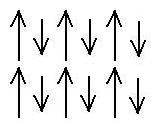
Anti-ferromagnetism is a bit more common than
ferromagnetism.
In this case, the adjacent moments do align in opposite
directions.
An example is NiO.
If an external B-field is applied to an anti-ferromagnet, what will
happen?
What will happen when the external field is turned off?
What will happen if the temperature of the anti-ferromagnet is raised?
The temperature at which this occurs is called the Neel temperature.
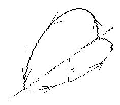
In ferrimagnetism, there are two (or more) types of magnetic
atoms which have different magnetic moments which are anti-parallel,
and
which therefor don't quite cancel:
This means that these materials can be very magnetic, and indeed, most
commercial ceramic magnets (like the ones on your refrigerator) are
ferrimagnetic.
In fact, out prototype natural magnet, lodestone (magnetite Fe3O4)
is
a
very complicated ferrimagnet, with three species of
magnetic
atoms, all iron. First, there are doubly ionized iron atoms which
occupy what are called 6-f sites in the crystal lattice, and there are
trebly ionized irons which occupy two different types of locations in
the
crystal lattice, 6-f and 4-f sites. A schematic of this system
might
look like this:
[Note: the notes on
dimagnetism are not
complete;
in particular, you should ignore the formulas, which still contain
errors!]
Unlike the effects list above, diamagnetism
is an orbital effect, rather than a spin effect. Here is a simple
classical model: Consider two electrons in the same orbital of an
atom. We consider them to be orbiting in opposite directions
(that
is, one has positive and the other negative orbital angular
momentum).
The magnetic moment of each is calculated from
m = IA = [q/t][pr2]
= [qv/d]pr2 = [qv/2pr]pr2
= qvr/2
and the directions of the moments are given by
the RHR, and so add to zero.
FIGURE
The centripetal force for each is provided by
the coulomb attraction from the positive nucleus:
keqQ/r2 = mv2/r.
Now, let's add a magnetic field B into the
page.
There will then be a magnetic force acting on each electron (qvB),
inward
on the clockwise moving electron (1) and outward on the
counterclockwise
moving electron (2); these additional forces change the centripetal
forces,
moving (1) into a tighter orbit and (2) electron into a bigger orbit:
keqQ/r12 + qvB
= mv2/r1
keqQ/r22 - qvB
= mv2/r2
We'll assume that v doesn't change, although
that may well not be true.
Continuing along this line requires solving a
messy quadratic, but all we need is to see that the two orbit radiuses
will be different, r1<r2. The magnetic
moment
due to orbital motion will be given by
m = IA = [q/t]pr2
= q[v/2pr]pr2
= qvr/2
So, m1 is
Since the radiuses of the orbits are now different, so are the magnetic
moments; the net magnetic moment actually points opposite to
the
applied magnetic field. As a result, the total magnetic field
inside
a diamagnetic material is reduced, in a manner similar to what happens
to the electric field in a dielectric. In fact, in the same way
that
conductors act to eliminate any electric fields in their interiors,
superconductors
are perfectly diamagnetic, so that the total magnetic field in a
superconductor
is zero.
Note:
There are, in fact, two
magnetic fields: the magnetic field proper, usually symbolized by H, and the magnetic induction field, B. While related, the two
fields represent different properties of magnetism. In this
class, we will deal almost exclusively with the induction field, B, but like almost everyone else, we
will refer to it incorrectly as the magnetic field.
Continue
on
to
the Next Section
Return
to
the
Notes Directory
D Baum 2001