Section 2-7 - AC Circuits
AC Resistor Circuit
RMS Values
AC Capacitor Circuit
AC Inductor Circuit
LC Circuit
Driven LRC Series Circuit
Maxwell's Equations
Correlation to your Textbook
AC Resistor Circuit
We've already discussed briefly in the last section the situation where
the emf in a circuit is not constant, as for a battery, but
rather
varying in time. Often, the variation is periodic and involves a
reversal of the direction of the emf. These emfs
cause
currents which alternate direction, and are therefor referred to as AC
currents (yes, it is redundant; 'AC' stands for alternating
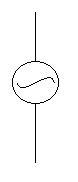
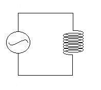
current). The symbol for such an emf
is
a circle with the waveform of the emf inscribed; for example a
sinusoidal
emf
is represented by
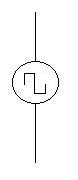
and a square wave emf should appear as follows.
We will concentrate on the sinusoidal emf for two reasons:
first,
it is fairly easy to work with mathematically, and second, just about
any
other shape curve can be approximated with a combination
of sine waves, so any general results we obtain should be true for
other waveforms as well.
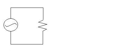
Let's consider a sinusoidal emf of the form e(t)
= emax
sin(wt
+ f) that is connected to a resistor:
Here, the phase angle f allows us to
change
the sine to a cosine or any combination of the two.
N.B.: We need to be very careful about the signs in the next few
sections.
e(t) = emax
sin(wt + f)
The voltage drop across the resistor is (by Kirchhoff's Loop
Rule) equal to the voltage rise across the emf source:
VR(t) = e(t)
so, VR = emax
sin(wt + f) = VRmax
sin(wt + f)
and by Ohm's relationship,
I = [VRmax/R] sin(wt + f)
= Imax sin(wt + f).
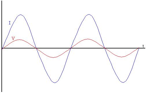
So, we find, very unsurprisedly, that the current through and the
voltage
drop across a resistor are in phase with one another, that is,
they
peak at the same time, are zero at the same time, et c.
RMS Values
Now, before we move on to the capacitor circuit, let's introduce some
new
terms. Consider the power dissipated in this resistor as thermal
energy;
instantaneously,
we have that
Pinstant = I2R = R[Imax sin(wt)]2 = R Imax 2
sin2(wt).
Note that here, I've dropped the phase angle term for simplicity; it
can always be replaced later.
Now, suppose that we want to find the average power
dissipated.
The average of the square of the sine (over one cycle) is 1/2.
We can see this easily by looking at the graph,
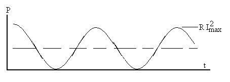
realizing that the area under the curve represents energy, mentally
cutting off the 'mountains' above 1/2R(Imax)2
and seeing that they fit exactly into the 'valleys,' forming a nice
straight
horizontal curve given by
Paverage = 1/2R Imax2.
Or, we can do this more mathematically: In general, the average
of a function over interval (a, b) is given by
FAVE = [ a b F(z) dz
]/[ab dz],
b F(z) dz
]/[ab dz],
so we get in this case (T = 2p/w is the
period of the cycle),
PAVE = [
0T R Imax 2
sin2(wt
+ f) dt
]/[0T dt]
= [
R Imax 2
1/w [1/2wt - 1/4 sin(2wt)] 0|T ]/[T]
= R Imax
2
1/wT [1/2wT - 1/4 sin(2wT)] = R Imax 2
1/wT [1/2wT - 1/4 sin(2w(2p/w))] = R Imax 2
1/wT [1/2wT - 1/4 sin(4p)] = 1/2 R Imax 2
.
Suppose that we ask what effective DC current would be necessary to
provide the same average power as this oscillating current does, i.e.,
Paverage = RIeffective2 ?
By comparing, we see that Ieffective = Imax/(2)1/2.
This particular result, called the r.m.s.,or
root-mean-square, current,
is valid only for the sinusoidal function. Other shaped curves
will
have different rms factors, which are calculated in the same way: we
took the
current,
squared it, averaged it, and then took the square root again.
We could have done the same thing with the voltage, finding that Vrms
= Vmax/(2)1/2, so that
Paverage = Vrms2/R = Vrms Irms.
The voltages and currents listed on household AC appliances are
actually
rms values: the given voltage standard of 110 VAC means that the
maximum voltage is about 155 V. A circuit breaker rated at 20 A
will
allow a peak current of 28.2 A.
Let's find the rms value of a square wave current:
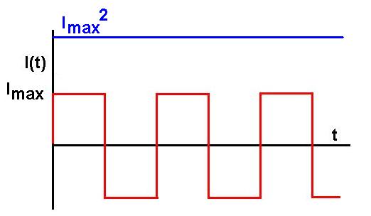
So this one is easy. Both the positive and negative portions
square to give Imax2. The average of this
is clearly Imax2, and the square root of that is
clearly Imax.
Try a harder one, the sawtooth wave:
The equation for the current is
I(t) = Imax [2t/T - 1] over the first cycle (other cycles
have similar expressions).
Square it:
I2(t) = Imax2 [4t2/T2
- 4t/T + 1]
Now, average over one cycle:
[ 0T Imax2 [4t2/T2
- 4t/T + 1] dt ]/[0T dt]
= Imax2
[ 0T [4t2/T2
- 4t/T + 1] dt ]/[T]
= Imax2
[[4t3/3T2
- 4t2/2T + t] 0|T
]/[T]
=
Imax2
[4T3/3T2 -
4T2/2T + T]/[T]
= Imax2
[4/3 - 4/2 + 1] =
Imax2/3
Then, take the square root to find the rms value:
Irms = Imax/(3)1/2.
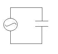
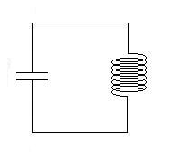
AC Capacitor Circuit
Consider a capacitor in series with a sinusoidal AC emf of the
form
e(t) = emax
sin (wt).
The voltage drop across the capacitor will be, by Kirchhoff's
Loop Law,
VC(t) = emax
sin (wt) = VCmax sin (wt).
But we also know that the voltage drop across the capacitor is q/C,
so let's find q(t):
q(t) = C VC = CVCmax sin (wt).
We'd like to to find the current, I(t), which we recognize as the rate
at which charge accumulates on the capacitor, I = dq/dt.
So,
I(t) = w CVCmax cos (wt).
This result tells us two very interesting things:
1) The current into the capacitor is not in phase with the
voltage
difference across it; in fact, we can say that the current leads
the voltage drop across the capacitor by 90o, or by one
fourth of a cycle:
2) We can write an expression resembling Ohm's Relationship between
the maximum current and the maximum voltage drop. We see from the
result that the maximum current is given by
Imax = w CVCmax ,
or
VCmax = [1/wC]
Imax.
The quantity [1/wC] is
somewhat similar
to the resistance in that it is a measurement of the degree to which
the
capacitor
inhibits charge flow in the circuit; its units will be ohms, just like
for resistance. Most interestingly, it will be frequency
dependent;
at low frequencies, very little current will be able to flow, while at
high frequencies, the current will be large. Since this quantity
looks useful, let's give it its own name and symbol: the capacitive
reactance,
cC
= 1/wC. Once again, just to
be very clear, the maximum voltage drop across the capacitor and the
maximum current do not
occur at the same time.
AC Inductor Circuit
Consider an inductor in series with a sinusoidal AC emf of the
form
e(t) = emax
sin (wt).
The voltage drop across the inductor will be, by Kirchhoff's
Loop Law,
VL(t) = emax
sin (wt) = VLmax sin (wt).
We also know that the voltage drop is actually an emf developed
across the inductor, e(t)
= - L dI/dt, so
the
voltage drop will be +L dI/dt.
So,
VLmax sin (wt) = + L dI/dt,
or,
dI/dt = [VLmax/L]
sin (wt).
We'd like to to find the current, I(t). Let's try integrating:
dI = [VLmax/L]
sin (wt) dt
I = [VLmax/L]
sin (wt) dt = - [VLmax/wL]cos (wt) +
Constant (the constant can be set to zero, since we have no
expectation of a DC component).
I(t) = - [VLmax/wL]cos (wt).
This result tells us two very interesting things:
1) The current through the inductor is not in phase with the
voltage drop across it; in fact, we can say that the current lags
the voltage drop by 90o, or by one fourth of a cycle.
2) We can write an expression resembling Ohm's Relationship between
the maximum current and the maximum voltage drop. We see from the
result that the maximum current is given by
Imax = [1/wL]
VLmax ,
or
VLmax = [wL] Imax.
The quantity [wL] is somewhat similar to
the resistance in that it is a measurement of the degree to which the
inductor
inhibits charge flow in the circuit; its units will be ohms, just like
for resistance. Most interestingly, it will be frequency
dependent;
at high frequencies, very little current will be able to flow, while at
low frequencies, the current will be large. Since this quantity
looks
useful, let's give it its own name and symbol: the inductive
reactance,
cL
= wL. Once
again, just to be very clear, the maximum voltage drop across the
inductor and the maximum current do not occur at the same time.
LC Circuit
Consider a circuit comprising a capacitor and an inductor, only.
Let's charge up the capacitor, then connect it to the
inductor.
Let's write a Kirchhoff's Loop Law equation to describe this.
Here we have the voltage drop across the capacitor on the left, and the
emf of the inductor on the right. For reasons which may
eventually become apparent, we'll define positive
q to be when positive charge resides on the lower plate of the
capacitor,
and positive current to be clockwise around the circuit. Then,
VC = eL
[1/C]q = - L dI/dt
+L dI/dt + [1/C]q = 0
+L d2q/dt2 + [1/C]q
= 0.
This is an equation we've seen before, and which we spent much time
and effort solving. Then, it was written
ma + kx = 0,
which is Newton's Second law written for a mass on a spring.
Remember that
v = dx/dt and
a = dv/dt = d2x/dt2,
so
m d2x/dt2 + kx = 0.
This equation is easily solved, but we will instead make use of the
analogy with the mass-spring system to figure out the behaviour of the
LC circuit. For a mass on a spring, the solution is:
x(t) = A cos(wot + f) with a natural frequency of oscillation wo = [k/m]1/2.
Which quantities in each system are analogous?
| displacement x |
charge on capacitor q |
| velocity v = dx/dt |
current in circuit I = dq/dt |
| acceleration a = dv/dt
|
dI/dt |
It appears that these are also analogous:
| mass m |
inductance L |
| spring constant k |
capacitance 1/C |
Does that make any sense? The mass is a measure of the system's
inertia,
that is, the how much the system would like to stay at rest (v=0) if
it's
already at rest, and stay in motion if it's already in motion.
The
inductance 'wants' to keep the current zero if it's already zero, and
maintain
its value if it's not zero. The capacitor, on the other hand,
always
tries to return the system to an equilibrium state, much as the spring
pushes the mass back toward the equilibrium point.
We can therefor guess that the solution to the LC circuit equation
is:
q(t) = qmax cos(wot + f) with wo
= [1/LC]1/2.
That is, every time this LC circuit is set in oscillation, it will do
so at this natural frequency.
In the mass-spring system, we saw that the energy changed form from
kinetic to potential, back to kinetic, et c. We already
know
from our discussions of RC and LR circuits that capacitors and
inductors
store up energy. If we take the expression for spring potential
energy
and substitute 1/C for k and q for x, we obtain
which we proved is the energy
stored in the capacitor. If we take the kinetic energy and
replace
m with L and v with I, we get
That is, the energy stored in an inductor is 1/2LI2,
as was asserted without proof in the last section, and which we have
now
shown through analogy. So, we see that the energy in an LC
circuit
is stored first in the electric field in the capacitor, then as
magnetic
energy in the inductor.
What else? The total magnetic flux in the inductor
is
fM
= LI, which is analogous to the momentum, p = mv.
Faraday's
Law, VL=+LdI/dt
then is analogous to the Newton's Second Law: F=mdv/dt.
The electric flux fE in the
capacitor
appears not to correspond directly with any quantity in the mechanical
example, but Gauss's Law for Electricity (the surface surrounds one
plate
of the capacitor) does appear to imply Hooke's Law:
fE = q/eo
eo[EA] = q
eoEA[d/d] = q
[eoA/d][Ed] = q
C[-V] = q
V = -[1/C]q => F = -kx
What if there had been a small resistor in the circuit? This
RI
terms plays the same role as a drag force, removing energy from
the system; after every half-oscillation, the capacitor charges up just
a little bit less. As the energy is removed, the oscillations (at
a frequency close to, but not quite equal to [1/LC]1/2) will
decay in amplitude.
Driven LRC Series Circuit
When we investigated the mass-spring system with drag, we discussed a
way
in which we could put energy back into the system. What was it?
Here, we will introduce energy by applying a driving emf, which
we shall assume is sinusoidal with frequency w,
which may well be different than wo.
Remember that, after a short period of combined frequency motion, the
system will eventually oscillate at the driving frequency.
We start with the notion that, in a series circuit, there is only
one
current, I, and that the voltage drops over the resistor, capacitor,
and
inductor must sum up to the voltage rise from the emf.
Now, we COULD try to solve this differential equation:
L d2q/dt2 + R dq/dt
+ 1/C q = emax
sin (wt + f).
Instead, let's
introduce a method by which we can easily keep track of what's going
on in the steady state.
Suppose that we wish to represent a function of the form
A(t) = Amax cos(wt).
Instead, we consider a phasor (A), a quantity which, like
a vector,
has magnitude but, unlike a vector, has phase instead of
direction.
The phasor A is
represented by an arrow, the length of which is
proportional
to the maximum value A can have. We plot the arrow on axes which
reperesent real and imaginary values (remember that
imaginary
numbers are multiples of the square root of minus one, called 'i' by
physicists
and mathematicians, 'j' by engineers).
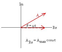
The quantity we are actually interested in is the projection of the
phasor along the real axis, or if you prefer, the real component
of the phasor. This is given by
Re
(A) = Amax
cos q.
To account for the oscillation in A, we will rotate the arrow around
the origin at frequency w, so that
q = wt
and
A(t) = Re (A) = Amax
cos wt.
To illustrate:
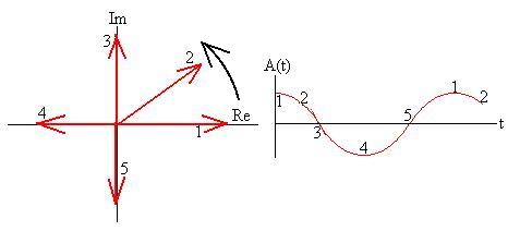
As the arrow turns counter-clockwise, the real component of the phasor
matches the actual value of A; at Point 1, A is at its maximum, as is
the
real part of the phasor; as time progresses to Point 2, the value of A
decreases as does the real component of the phasor, until each is zero
at Point 3, and so on.
Let's use this method to construct a phasor diagram for what's
happening
in the driven LRC series circuit and, from it, derive some useful
relationships.
We'll actually construct the diagram backwards, in the sense that we'll
start with the current and end with the emf, even though in
reality,
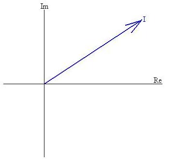
the emf drives the current. Pick a phase for the current
I,
keeping in mind that the arrow will rotate around the origin at
frequency
w:
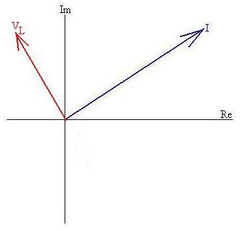
We already worked out the phase relationships between the current and
each of the voltage drops. For example, we said that the current
through the inductor lags the voltage drop by 90o, so we
should
draw in the inductor's phasor 90o ahead, or
counter-clockwise,
of the current's phasor:
where, again, the length of the arrow tells us the maximum value of
that voltage drop, with VLmax = wL
Imax. Let's put in phasors for VR (in
phase
with I) and VC (90o behind I):
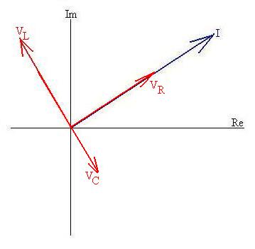
Keep in mind that this is a generic diagram; we have no idea how long
to make the arrows. Also remember that the whole system of arrows
is rotating counter-clockwise with frequency w.
From Kirchhoff's Loop Law, we know that e
= VL + VC + VR, and so we can say that
this is true of the phasors representing them as well, since
e = emax cos(wt) Here, f
is the as yet unknown angle between the emf and the current.
VL = VL max cos(wt + p/2)
VR = VR max cos(wt)
VC = VC max cos(wt - p/2).
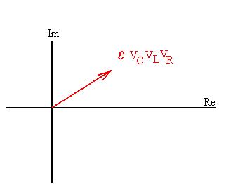
So, we can put in the phasor representing the emf as the
'phasor
sum' of the voltage drops:
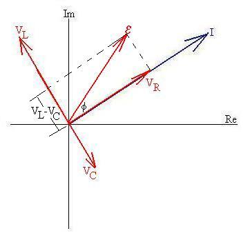
Since VL and VC are in opposite 'phases,' the
component of the emf in that 'direction' is VLmax - VCmax,
where we remember that VCmax could very well be larger than
VLmax, in which case the emf would be on the other
side
of I, i.e., lagging behind I.
Now, we can work out some interesting relationships:
tanf = [VLmax - VCmax]/VRmax
= [cLImax - cCImax]/RImax
= [cL - cC]/R
= [wL - 1/wC]/R.
tanf = [wL -
1/wC]/R.
emax =
[VRmax2
+ (VLmax - VCmax)2]1/2
=
[(RImax)2 + (cLImax
- cCImax)2]1/2
= [(R)2 + (cL -
cC)2]1/2
Imax
Here we once again have a relationship which looks a little like Ohm's
Relationship. Let's give the quantity in brackets its own name,
the
impedance
Z:
Z = [(R)2 + (cL
- cC)2]1/2
so that
emax = Z
Imax
Keep in mind that the maximums in the emf and the current will
generally not occur at the same time.
We can see that the amplitude of the current in the circuit will be
greatest when Z is smallest, and that will occur when
cL - cC
= wL - 1/wC = 0,
or when w = [1/LC]1/2 = wo.
So, just as for the mass-spring system, the greatest response will
occur when the driving frequency matches the natural frequency, a
condition
refered to as resonance.
In that situation, Z = R, and f = 0, and
the circuit behaves as if it were purely resistive (i.e., emax
= R Imax and e
and I are in phase), since the capacitive and inductive effects cancel
each other exactly.
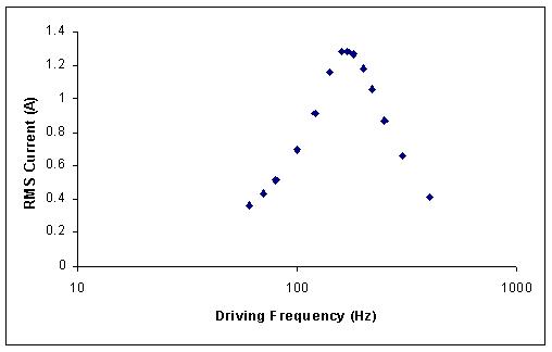
Here are the results of measurements on an RLC circuit with L = 8.3mH,
C = 100mF, and R = 5.5W.
The maximum amplitude current occurs (as predicted) when the driving
frequency
is fo = 1/[2p(LC)1/2]
= 175 Hz.
What power is dissipated in this circuit? The energy leaves as
thermal energy through the resistor, and the instantaneous energy lost
there is
Pout = VR I.
The average power (assuming sinusoidal functions) is then
Pout average = 1/2 VRmax Imax
=
VRrms Irms.
From the diagram above, it should be clear that
emax = VRmax
cosf,
so that
Pout average = 1/2 emax
Imax
cosf
=
erms
Irms
cosf.
These expressions of course also represent the power into the circuit
in the steady-state situation. The cosine term is often referred
to as the power factor of the circuit.
Mastery Question
Find the impedance as a function of frequency for a
driven LRC parallel circuit. Click
here
for a solution.
Additional Neat Note
You can probably imagine that combinations of inductors,
capacitors, and resistors can be used to build analog circuits that
will output the derivatives or intergrals of mathematical functions, so
long as those functions can be represented by a time-varying
voltage. Do a Google search in your free time.
Maxwell's Equations and EM Waves
Let's return briefly to Ampère's law:
 B|| dl
= moIencl
B|| dl
= moIencl
Consider a wire carrying current I and a point P at which we want to
find the magnetic field caused by that current. We draw a loop
around
the wire and evaluate the integral on the left hand side of
Ampère's Law,
and
find that the result is proportional to the current enclosed by the
loop.
How exactly do we determine if a loop encloses a current or not?
One way is to consider a surface (yellow in the figure below) that is
bounded
by the loop; if the current penetrates from one side of the surface to
the other, then the loop encloses the current.
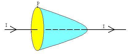
However, there can be many surfaces bounded by a given loop.
Consider for example the blue surface in the upper figure. Since
the current I also passes from one side of the blue surface to the
other,
we should get the same result for the field at P.
Now, place a capacitor in the wire as shown below.
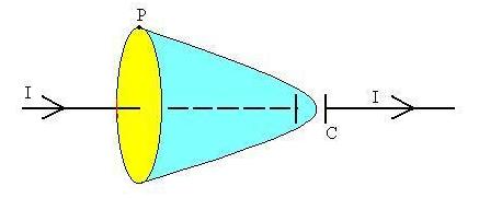
Let's calculate B at P again. Using the yellow surface, we arrive
at the same answer as above, but using the blue surface, we get zero,
since
there is no current pentrating the surface.
Maxwell (see note) recognized this problem and
postulated that the changing
electric
field between the plates of the capacitor might also be responsible for
causing magnetic fields. He modified Ampère's Law in the
following
way:
B|| dl
= moIencl
+ moeo dfE/dt.
Let's investigate further (assuming all of our approximations for a
parallel plate capacitor hold true):
fE = EA = [s/eo]A
= [Q/Aeo]A = Q/eo
Not surprising, considering Gauss's Law for Electricity and the fact
that the E-field is zero except between the plates of the
capacitor.
Then the extra term becomes:
moeo
dfE/dt
= moeo d[Q/eo]/dt
= mo dQ/dt
= mo I.
This flux term, eo dfE/dt,
is then numerically equal to the real current in the wire and is
referred
to (for historical reasons) as the displacement current.
The set of four equations we have been working with are now
collectively
known as Maxwell's Equations:
 Eperp
dA
= qencl/eo
Gauss's Law for Electricity
Eperp
dA
= qencl/eo
Gauss's Law for Electricity
Bperp
dA
= 0 Gauss's Law for Magnetism
E|| dl
= (-) dfM/dt
Faraday's Law of Induction
B|| dl=
moIencl + moeo dfE/dt
Maxwell's modified version of Ampere's Law
Maxwell's contribution tells us that, in much the same way that a
changing
magnetic field can cause an electric field, a changing electric field
can
create a magnetic field. Before we discuss the incredible
importance
of this notion, we need a little background.
Mechanical waves obey a specific differential equation
called
the wave equation (we worked this out for transverse waves on
a string in PHYS 1):
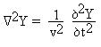
Y represents some quantity's deviation from an equilibrium value (such
as the transverse displacement of a string) and v represents the speed
of the wave. For the case of wave on a string, it can be
shown
fairly easily that this corresponds to a combination of Hooke's Law and
Newton's Second Law (e.g.,
d2Y/dt2
is the transverse acceleration, 1/v2 is proportional to k/m,
et
c.).
If we take somewhat more mathematically sophisticated versions
of the Maxwell equations and combine them, we obtain two wave
equations:
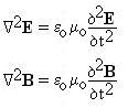
along with some other interesting results. There is a very good
algebra-based derivation of this result in Weidner and Sells, Elementary
Classical Physics, Allyn and Bacon, Boston (1973).
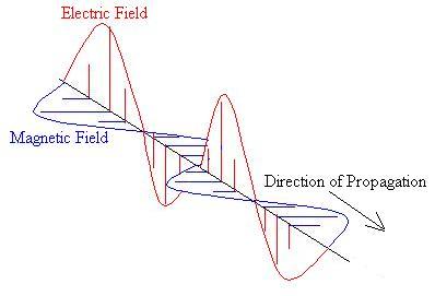
The implication is that it may be possible to have electro-magnetic
waves, which travel through vacuum with speed
v = 1/(moeo)1/2.
However, the E and B fields must be at right angles to each other and
to the direction of propogation of the wave (in fact, v is
parallel
to E x B), and at any point,
B = E (moeo)1/2.
In addition, the wave carries energy with an average intensity
of
Iave = E B/2mo
Calculate the speed of these EM Waves in vacuum, given that v = 1/(moeo)1/2.
We'll discuss the implications of this result in the next section.
Note
Maxwell did this interesting work, but presented his results in a very
complicated mathematical framework. We usually credit Heaviside
with the present formulation of the equations.
D Baum 2001, 2003