So long as the speed of an object is less than about 10% of the speed of light, and the object is larger than an atom but smaller than a star, we will probably be alright.
Aristotle is the earliest
identifiable
author on the topic of physics (384-322 B.C.). He is often
referred
to as the first observational physicist, since he based his notions on
what he saw in everyday life around him. We discussed the dangers
of Aristotelian thought, which is based on logical argument, but often
on false premises, leading to false conclusions. An example might
be:
Travelers walk more quickly when
they draw near their destinations.
Falling objects travel toward the
earth.
Therefore, falling objects speed
up as they fall toward the earth.
An argument is sometimes made that
Aristotle was more interested in using natural science as a vehicle to
sharpen his logical skills than in determining the workings of the
universe.
A great number of physicists worked between the time of Aristotle and 1600 (see Rene Dugas, Histoire de la mecanique, Editions du Griffon, Neuchatel (1955) for a fascinating read), but we shall ingore them and instead talk breifly about Galileo. Galileo is now considered to the the first experimental physicist, in that he set up situations where he could control and vary conditions in order to separate out the various effects acting on a moving object. For example, we discussed the case of a book sliding on a tabletop and coming to rest. Aristotle might have said that the book came to rest because rest is its natural state. Galileo might have said that the book would have continued to move at constant velocity, but was slowed by friction. He might have demonstrated this by making the tabletop smoother and smoother and noting that the book traveled further each time. We credit Newton with synthesizing much of Galileo's and others' work into a coherent picture.
We spoke of how physics can be considered to be a constructed logical system, which must be self-consistent, and consistent with objective reality. Goedel showed that logical systems can not be both closed and self consistent. In the case of plane geometry, for example, there are five axioms which are assumed to be true without proof. If we think of physics as a logical system, then there must be axioms or premises on which the system is based which are independent of the system itself. These premises we call laws. Modern physics is based on observation and experimentation which allow us to formulate these laws, which are things we never have seen to be untrue and we therefor assume are always true. We can test them both directly and by testing the derived implications in which they result; any inconsistency between reality and these implied conclusions suggests that the premises on which the conclusion was based may be false.
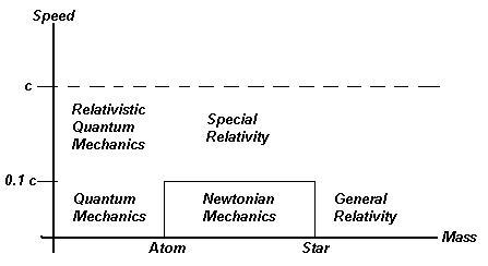
In this semestre, we will study
what
is now known as Newtonian mechanics. The laws we shall
discuss
are unfortunately only approximately true, special case limits of the
actual
laws of the universe. However, they are sufficiently correct to
agree
to high precision with reality so long as certain conditions are
met.
The diagram below shows a rough breakdown of the approaches necessary
to
a given situation.
So long as the speed of an object
is less than about 10% of the speed of light, and the object is larger
than an atom but smaller than a star, we will probably be alright.
Dimensional analysis can be a useful tool for gaining insight into the relationships among quantities which determine the behaviour of a system. For example, can we make a prediction for the dependence of the period (T, the time to complete one cycle) of a simple pendulum with out knowing much physics? On what could this depend? Perhaps the length L of the string, the mass M of the bob, the amplitude of oscillation (qA, the angle through which the bob swings), and perhaps the earth's gravity g, whatever that is. What are the dimensions of these quantities?
period T = [Time]
mass M = [Mass]
string length L = [Length]
amplitude qA
=
[1] (dimensionless)
gravitational field strength g =
[Length]/[Time]2 (O.K., I had to give you this one).
What combination of T, M, L, qA,
and g will result in [Time]? Well, we won't need the mass, since
wherever we stick it in, we have to cancel it back out again. The
only place to get [Time] is from gravity, but since it's on in the
denominator,
and squared, we'll have to invert g and take its square root:
Dimension of g-1/2 =
[Time]/[Length]1/2.
But we also have to eliminate the
length term, and we can do that by multiplying by the square root of
the
string length:
Dimension of L1/2g-1/2
= [Length]1/2 [Time]/[Length]1/2= [Time].
Now, what about qA?
Since it's dimensionless, it might go anywhere. But if we try a
little
experiment, we find that qA
in fact has no effect on the period. So, our final result is that
we expect the period of a simple pendulum to go as
T = [L/g]1/2.
The correct answer, as we'll see
in December after much toil is
T = 2p[L/g]1/2.
Since 2p
is a dimensionless quantity, this method could not detect it.
Even
so, we got a good idea of how the period depends on the
parameters
of the system with relatively little work.
Here's another one: If we
drop
a marble from a height H above a table, it takes a certain amount of
time
to fall through distance H to the table. Can we work out roughly
the relationship between the time t and the height H?
What quantities might affect the
time and what are their respective dimensions? Well, we have
height H = [Length]
time t = [Time]
mass m = {Mass}
gravitational field strength g =
[Length]/[Time]2
inch;
foot; 1 foot = 12 inches
yard; 1 yard = 3 feet
fathom; 1 fathom = 2 yards
rod; 1 rod = 16 2/3 ft
ell; 1 ell = 2 ft
mil; 1000 mils = 1 inch
furlong; 1 furlong = 220 yards
chain; 1 chain = 66 feet
link; 100 links = 1 chain
mile; 1 mile = 5280 feet = 1760
yards = 8 furlongs
league; 3 miles = 1 league
hand; 1 hand = 4 inches
span; 1 span = 9 inches
palm; 1 palm = 3 inches
finger; 1 finger = 7/8 inch
digit; 1 digit = 1/16 foot
shaftment; 1 shaftment = 6 inches
Even worse, a historical inch in Brunswick may not be the same as an inch in some other part of Europe.
We can see that the conversion factors are also unwieldy. The U.S. is one of only two nations to use the English system (Burma is the other), in spite of the fact that the conversion was to have been accomplished by 1970. Metric road signs are in use on only a few federal highways. See this link for more information.
Let's examine some weight measurements:
Which weighs more, a pound of
rocks
or a pound of feathers?
Which weighs more, an ounce of
gold
or an ounce of potatos?
Which weighs more, a pound of
gold
or a pound of potatos?
The metric system survives as one
of the innovations of the French Revolution (the calendar was not so
lucky,
but then how would we know when not to eat oysters?). There is a
small number of basic units, and all other units with the same
dimension
are some power of ten larger or smaller, usually specified with a Latin
or Greek prefix:
giga = 109
mega = 106
kilo = 103
milli = 10-3
micro = 10-6
nano = 10-9
et c.
For example, the metre is
the basic unit for length, and other units include the kilometre (1000
m), the milllimetre (1/1000 m), et c.
The definitions of each unit are also well specified, although many definitions have evolved. For example, the metre was initially defined in the 1790s as 1/10,000,000 of the distance from the equator to the North Pole along the meridian passing through Paris. Since this is not an easy standard to use, it was redefined in 1889 as the distance between two scratches on a platinum-iridium bar, kept just outside Paris. Since taking a long trip to compare measurements with the bar is inconvenient, each major nation was provided with its own bar (ours is in Gaithersburg). As the necessity of making more precise measurements increased, the definition of the metre was changed so that anyone with the proper equipment could reproduce the standard; in 1960, the definition was changed to the distance covered by a 1,650,763.73 wavelengths of a particular orange emission line generated by 86Kr. Finally, the definition of the metre was changed again in 1983 to be the distance traveled by light in 1/299,792,458 of a second.
Although it seems as if the progressive definitions of the metre are making it more difficult to compare our measurements to the standard, it is actually the reverse; by liberating the standard from a particular piece of matter and basing it more on the laws of the nature, which are universal, anyone with the appropriate equipment can reproduce the standard in the comfort of his own laboratory. The only standard which has not yet been so liberated is that of the kilogram; a recent article in The Baltimore Sun told of how the U.S. standard kilogram is slowly losing mass.
Students often find converting
units
difficult. Here is the Factor Label Method, which you may
find useful. Suppose that we wish to find out how many seconds X
there are in 3 years:
X seconds = 3 years
Note that the units are different
on each side, but that the dimensions are the same, [Time].
We'll multiply the right hand side
of the equation by a quantity equal to one; we do that because
multiplying
a number by one does not change its value. The quantity we choose
to multiply by is (12 months/1 yr). Since the numerator equals
the
denominator and since both have dimensions of [Time], the quotient
equals
one, and the right hand side is still equal to three years:
X seconds = (3 years)*(12 months/1
year).
Canceling the units and doing the
multiplication results in
X seconds = 36 months.
A complete calculation might look
like this:
X seconds = (3 years)*(12
months/1 year)*(30 days/1 month)*(24 hours/1 day)*(60 minutes/1
hour)*(60
seconds/1 minute).
So, years cancel years, months
cancel
months, et c., to obtain 3*12*30*24*60*60 seconds =
9.33x10⁷
seconds.
Try this:
A metre is 100 centimetres.
Find the volume in cubic centimetres of a box with a volume of one
cubic
metre.
Theories in physics are required to agree with reality to at least some degree. Once a theory has been developed, it is necessary to conduct experiments to verify the predictions of the theory or to find a counterexample disproving it. Accurate and precise measurements of the attributes of objects in the real world are therefor required. However, the exact value of any one of these attributes can never be known. Each measurement X should therefor be accompanied by an estimate of how well the experimenter thinks he knows the value, or alternately, how confident he is that the value is correct, the uncertainty: X ± dX. There are many different ways of doing these estimates, some quite complicated, mathematically. We will concentrate on a couple of them only. It should also be noted that, on occasion, experiments can be designed with the intention of reducing uncertainty; an example will be given in class.
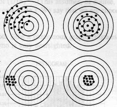 Let's take a
moment to discuss the differences between precision and accuracy. A naïve
distinction might be as follows: accuracy is a measure of
how close the result is to the (presumably unknown) correct answer,
while
precision
is a measure of how reproducible the measurements are. Here is an
illustration
of the difference using the example of target shooting. The
bull's
eye represents the 'correct' answer, which we probably do not know. The
bullet holes represent the measurements made by an experimenter. Try to
determine which diagrams correspond to high precision and to high
accuracy.
Let's take a
moment to discuss the differences between precision and accuracy. A naïve
distinction might be as follows: accuracy is a measure of
how close the result is to the (presumably unknown) correct answer,
while
precision
is a measure of how reproducible the measurements are. Here is an
illustration
of the difference using the example of target shooting. The
bull's
eye represents the 'correct' answer, which we probably do not know. The
bullet holes represent the measurements made by an experimenter. Try to
determine which diagrams correspond to high precision and to high
accuracy.
Once the uncertainty of a measurement is calculated (see below), it should be reported in a very particular format. The uncertainty should be rounded to one significant figure, and the value itself should be rounded to the same place as the uncertainty. As an example, suppose that a student calculates a value of 23.4037 units with an uncertainty of 0.00452 units. The uncertainty dX will round to 0.005 units and the value itself will round to the thousandths place, X = 23.404. The reported value then will be 23.404 ± 0.005 units.
The manner in which the uncertainty is determined depends on many factors, such as the number of measurements made, the type of device being used (e.g., analog or digital), whether the value changes with time, et c. It should also be made certain that the measuring device is properly calibrated. Some of the more common situations are listed here:
If only one measurement is feasible,
Here are two examples: for each set of numbers, find the mean, the standard deviation, and the uncertainty.
| Example I | Example II |
| ESU = 0.0333 cm | ESU = 0.0333 cm |
| 57.03 | 57.03 |
| 57.10 | 57.00 |
| 57.10 | 57.06 |
| 57.00 | 56.97 |
| 57.03 | 57.00 |
| 56.93 | 57.03 |
| 57.07 | 57.00 |
| 57.07 | 57.00 |
| 57.00 | 57.00 |
| 56.93 | 57.00 |
| Average = ? | Average = ? |
| St Dev = ? | St Dev = ? |
| Uncertainty = ? | Uncertainty = ? |
Often, the result desired is calculated from measurements of several different quantities. For example, a student may wish to know the volume of a rectangular block, V ± dV from three edge length measurements, A ± dA, B ± dB, and C ± dC. A quick calculation, assuming that the uncertainties aren't too large, shows that the maximum value for dV is (AB dC + AC dB + BC dA). However, this assumes that the measurements were all either over - or under- estimated, when of course one could be over and another under, thereby canceling their effects. What we really want is the most likely uncertainty. The process by which the uncertainty of a calculated quantity is found is called propagation of uncertainty. The mathematical process with which these calculations are rationalized is beyond the scope of this course, but we can certainly make use of the results for common cases:
Find the density of a cylinder.
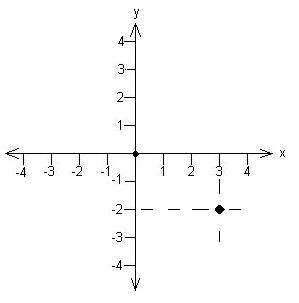
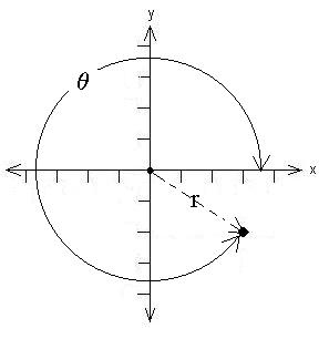
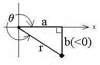
| x = r cosq y = r sinq |
| r = + (x2 + y2
)1/2 and q = arctan (y/x) |
In our example, r = [32
+ (-2)2]1/2 = 3.61 and q
= arctan[(-2)/3] = -33.7o. Now, as stated
above,
we have to worry about whether the answer obtained from the
calculator, which can't distinguish arctan[(-2)/3] from arctan[2/(-3)],
is in the correct quadrant; we want an angle in the fourth quadrant
because
our x value is positive and the y value is negative. So, -33.7o
or +326.3o is the correct answer.
Let's double check by reverse
converting:
x = r cosq = 3.61*cos(326.3o)
= 3.003 (close enough), and
y = r sinq = 3.61*sin(326.3o)
= - 2.002.
Try it: Find the polar
co-ordinates
for the cartesian location (-1, 3).
A scalar is a quantity with only magnitude (e.g.,
temperature).
A vector is a quantity which has both magnitude and direction
(e.g., wind velocity).
Are there other types of quantities? Yes, the next one up is
called a tensor, followed by super tensors, super-super
tensors, et c.
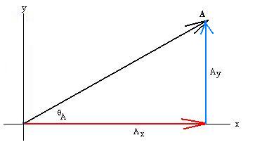
The names of vectors are written in bold type in print, or with an
arrow when handwritten: A or  .
The magnitude of a vector is denoted by dropping the bold type, or by
enclosing
the symbol with vertical lines: A or |A|.
.
The magnitude of a vector is denoted by dropping the bold type, or by
enclosing
the symbol with vertical lines: A or |A|.
For now, it might be useful to visualize vectors specifically to represent displacements, while realizing that they may also represent much more abstract quantities. So, in that sense, the vector A tells us to travel so far in such-and-such a direction. An example might be 5 km at qA=37o, remembering that the angles are customarily measured CCW from the x-axis.
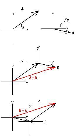
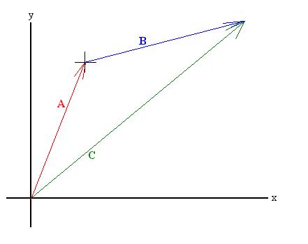
We can visualize adding vectors again in terms of displacements: A
+ B says that we should start at our origin and travel A m in a
direction given by qA, then from
that intermediate destination, travel B m in the direction given by qB.
Conceptually, this is known as the tip-to-tail method of addition:
We can move the vectors around at our convenience to add them as shown,
since a vector is defined only by its magnitude and direction; so long
as those are kept the same, we can slide the vector around the page as
much as we want.
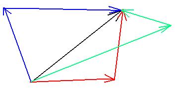
We realize that addition is commutative (see figure above) and
associative
(not shown). The vector A + B can be given its
own
name (C?) so that we can write that
C = A + B = B + A.
C is called the resultant of the addition of A and
B. Here is an equivalent alternate method, called the parallelogram
method of addition:
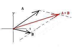
Place the vectors tail to tail, then construct lines parallel to each
through the tip of the other. The diagonal is then A + B.
You can see how these methods are identical: the lower triangle
corresponds
to the one in the B + A figure above, while the upper
one
corresponds to the A + B figure above.
Subtraction of vectors is not obvious, but we can take a leaf from
the
algebraists' notebook:
A - B = A + (-B),
where (-B) is a vector with the same magnitude as B,
but directly oppositely.
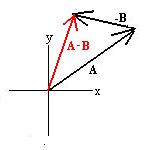
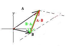
Comparison to the parallelogram method reveals that A - B
is the other diagonal of the parallelogram (as is B - A
pointing
in the opposite direction):
To add vectors graphically, one would take paper, ruler and protractor,
choose a scale, and draw arrows to represent the vectors such that the
length of each is proportional to the magnitude of the corresponding
vector.
To find the resultant, measure the length of the resultant with the
ruler
and back convert to find the magnitude, and use the protractor to find
the direction.
Now, we have an alternate manner of adding vectors using the
components.
Let C = A + B:
Let's draw in the components of both A and B, as well as of C:
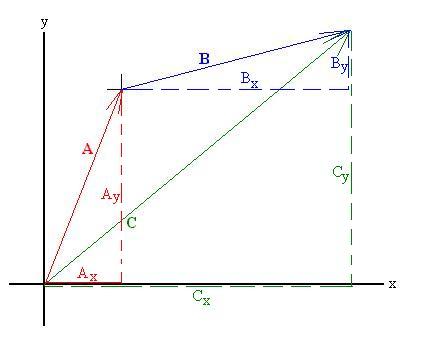
It should be clear that Cx = Ax + Bx
and that Cy = Ay + By. We might
say that the each component of the sum of two vectors is the sum of the
corresponding components of the two vectors. Subtraction of
vectors
works the same way.
Converting C back into a magnitude and direction is easy:
Use
the Pythagorean theorem to find |C|:
C = [Cx2 + Cy2]1/2
and qC = arctan[Cy/Cx].
Be sure to watch the quadrant!
It might be useful to introduce vector multiplicaton
at this
point. There are several types of multiplication, of which we
will
discuss two.
We define the scalar product (also called the inner
product
or the dot product) of two vectors A and B to
be:
A.B
= |A| |B| cosqA,B,
= ABcosqA,B,
that is, the magnitude of A times the magnitude of B times the cosine
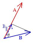
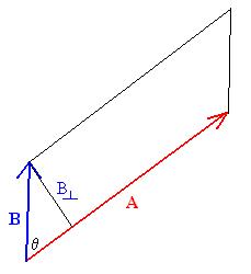
of the angle between them. One interpretation of this definition
is that we are multiplying the magnitude of A vector by the
component
of B that lies in the direction of A:
A.B
= AB|| = A(BcosqA,B).
Using the unit vector notation form above, we first realize that we
have that
i . i =
j . j = k .
k = 1
since for each pair, the vector magnitudes are 1 (and dimensionless)
and the angle between paired vectors is 0o,
and that
i .
j = j .
i = j
. k = k .
j = k .
i = j .
k = 0,
since each of these paired vectors are perpendicular to each other.
A.B = (Axi + Ayj + Azk) . (Bxi + Byj + Bzk) = AxBx + AyBy + AzBz
Another type of vector multiplication is the vector product or
the cross
product: A × B. We define the
magnitude of the cross
product to be
|A × B| = |A| |B| sinqA,B,
= AB sinqA,B.
The direction of A × B is perpendicular to the
plane that
contains A and B and can be obtained by using the right-hand-rule
(RHR). Point the index finger of the right hand in the direction
of A and the middle finger in the direction of B; the
right
thumb then points in the direction of the cross product. One
interpretation
of the cross product's magnitude is that it is the area of the
parallelogram
formed by the vectors A and B when they are placed tail
to
tail:
The base of the parallelogram is A and the height is Bsinq,
making the area A(Bsinq). What is the
direction of A × B in this example?
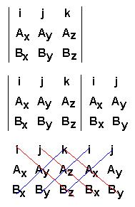
A × B = (Axi + Ayj + Azk) ×
(Bxi + Byj + Bzk) = (AyBz - ByAz) i + (AzBx - BzAx) j + (AxBy -
BxAy) k