vector r point from the origin to the location of the object. If the object moves, then there will be an initial position vector, ri, and a final position vector, rf. The difference between them will be Dr.

We'll need first of all to be
able to define the location or position of an
object. We talked in the last section about how to
describe the location of an object in terms of its x-, y-, and
z- co-ordinates. Alternately, we can describe the position
using spherical co-ordinates, using r, q, and f. Let
the
vector r point from the origin to the location of the
object. If the object moves, then there will be an initial
position vector, ri, and a final position vector, rf.
The difference between them will be Dr.
The vector Dr is
called the displacement; it depends only on the initial position and
the final position, and not on the path the object took between
them.
Suppose that the blue line
represents the actual path taken by the object:

The distance is the
length of the actual path taken. Distance is a scalar
quantity. Consider three scenarios: 1) the object moves in
a straight line from its initial to its final position; 2) the
object moves along the blue line shown; 3) the object takes a
trip to the moon and returns to earth to end at its final
location. While the distances in each case are different,
the displacement in each case is the same as for the other
situations. Note this special case, however: if the object
travels along a straight line, the distance and the magnitude of
the displacement are the same value.
The average speed
is defined as the distance traveled per unit time, or speed = s/Dt.
We can can also talk about the instantaneous
speed:
inst speed = limit Dt->0
s/Dt.
Now, we see that when the time interval becomes sufficiently
short, the object has no opportunity to deviate from a straight
segment on its path. In that case, as discussed above, the
distance and the magnitude of the displacement become equal. So,
inst speed = limit Dt->0 s/Dt = limit Dt->0 |Dr|/Dt = limit Dt->0 |Dr/Dt| = |vinstantaneous|.
So the instantaneous speed is the same as the magnitude of the
instantaneous velocity.
We define the average acceleration as the change in
velocity per unit time:
aave = Dv/Dt,
and the instantaneous acceleration as
ainst = limit Dt->0Dv/Dt = dv/dt = d(dr/dt)/dt = d2r/dt2.
The analysis is the same for a as it was for v, so the work will not be repeated here.
We can continue the process indefinitely. For example, the
average jerk is defined as
Jave = Da/Dt,
and the instantaneous jerk is
Jinst = limit Dt->0Da/Dt = da/dt = d3r/dt3.
and so on with the kick and then the lurch.
Then,
vinstantaneous = limit Dt->0Dr/Dt = dr/dt.
ainstantaneous = limit Dt->0Dv/Dt = dv/dt
= d2r/dt2.
Jinstantaneous = limit Dt->0Da/Dt = da/dt
= d3r/dt3.
Kinstantaneous = limit Dt->0DJ/Dt = dJ/dt
= d4r/dt4.
Linstantaneous = limit Dt->0DK/Dt = dK/dt
= d5r/dt5.
And, of course, there's no reason to stop there.
Start with the definition of the acceleration. Since the
acceleration is constant, that value is also the average
value. So,
aAVE = a = Dv/Dt = [vf - vi]/[t
- ti] = [v - vi]/t,
which re-arranges to
v = vi + at. (1)
Again, this is true if the acceleration is constant.
Next, we'll start with the definition of the velocity,
v = dr/dt
dr = v dt
Eq (1) gives us the velocity as a function of time, so we can
substitute:
dr = (vi + at)
dt.
Next. we'll integrate, making sure that the limits of integration
for each match, i.e. we start at ri at
t = 0, and end at rf at time t.
ri![]() rf
dr = 0
rf
dr = 0![]() t (vi
+ at) dt.
t (vi
+ at) dt.
Dr = rf - ri
= vit + 1/2 at2
Or, in its final form,
r = ri + vit + 1/2
at2 (3)
Next, we'll combine two definitions: v = dr/dt
and a = dv/dt.
Let's take the dot product of the left side of each equation with
the right side of the other:
v . dv/dt
= a . dr/dt
v . dv =
a . dr
v dv = a
. dr
N.B.: This step may seem a bit iffy, but I can show you the
process from one step to the next that justify it.
Let's integrate, again being sure that the limits on each side
correspond. Remember we're requiring that a is
constant, so it can be pulled out of the integral.
vi![]() vf v dv = a
. ri
vf v dv = a
. ri ![]() rf
dr
rf
dr
1/2 v2 vi|vf
= a . Dr
vf2 - vi2 = 2 a
. Dr
or, in its final form,
v2 = vi2
+ 2 a . Dr (4)
Now,
let's swing back for Eq (2).
vaverage
= Dr/Dt = Dr/t
Remember, we're setting ti to 0.
From (3), we know that Dr =
vit + 1/2 at2,
so let's substitute:
vaverage = [vit
+ 1/2 at2]/t
= vi + 1/2 at
= 1/2[2vi + at]
= 1/2[vi + vi
+ at]
From (1), v = vi + at,
so substitute:
vaverage = 1/2[vi
+ v]. (2)
Alternatively, we can do some out of the box thinking.
Consider the v(t) graph below:
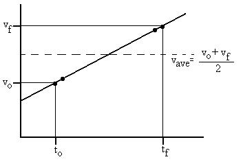
The curve is a straight line, because the acceleration is constant
and is represented by the slope of the curve; it may well have
been a negative slope, or even a zero slope, instead of the
positive slope pictured here. We need to average the
infinitely many values the velocity has in the interval ti
to tf.
Now, we have four kinematic equations that are valid in the special case of constant acceleration:
| v = vi + at vave = [vi + v]/2 r = ri + vit + 1/2at2 v2 = vi2 + 2a. (r - ri) |
Various combinations and perturbations of these should allow for solving most problems. Here, however, is a warning: do not rely on the equations by themselves to solve problems. The equations are in a sense tools, but it still requires the brain to direct their use.
Continuing along in a
similar manner for other quantities, the relationships above
become:
v = dx/dt
a = dv/dt
v = vi + at
vave = [vi + v]/2
x = xi + vit + 1/2at2
v2 = vi2 + 2a
Dx
Notice that the dot product was dropped from the last equation. This will still work out if we use the following convention. Since the displacement, velocity, and acceleration are indeed all vectors, we need a mechanism to describe their directions. So, let's say that if the velocity is to the positive x direction, we'll insert a positive value in for v in the equations, and if the velocity is pointed in the negative x directions, we'll insert a negative number. Same for the acceleration. Now, if the accelerationand displacement ar ein the same direction, whether both positive of negative, the dot product would give us a positive result. Contrarily, if they were in opposite directions, we'd obtain a negative value. This convention maintains those results. (=)(+) = (-)(-) = (+) and (+)(-) = (-)(+) = (-).
OK, now, let's work through some 1-d examples to help firm up your understanding.
Examples: Suppose that
an object starts out at xi = 3 and ends at xf =
5, and makes that trip smoothly and without reversing
direction. What is the displacement? Now, suppose
instead that the object travels from x = 3 to x = 15, then back
to x = - 8, then on to x = 5. What is the displacement in
that case?
Distance (s) is the term we use for the length of the path
taken. So long as the direction of motion doesn't change,
the distance is the same as the magnitude of the displacement.
Examples: Suppose that an
object starts out at xo = 3 and ends at xf =
5, and makes that trip smoothly and without reversing
direction. What is the distance? Now, suppose
instead that the object travels from x = 3 to x = 15, then back
to x = - 8, then on to x = 5. What is the distance in that
case?
Find the average speed in these examples.
Suppose that an object starts
out at xi = 3 and ends at xf = 5, and
makes that trip smoothly and without reversing direction in 3
seconds.
Suppose instead that the object
travels from x = 3 to x = 15, then back to x = - 8, then on to x
= 5, all in 3 seconds.
Try another example:
Jimmy walks across the room (10
m) in 10 seconds, and runs back in 5 seconds.
What is his displacement?
A distracted driver traveling at 15 m/s notices a stop sign when he is 10m from the stop line. If the car decelerates at 6 m/s2, how quickly is the car moving as it passes the stop line?
Let's write down the quantities which we know either implicitly
or explicitly, as well as what we want to figure out:
xi = 0 (start at the origin)
xf = 10 m
vi = 15 m/s
vf = ? (We would like to know this.)
a = - 6 m/s2 (a deceleration of 6 m/s2 is
an acceleration of -6 m/s2, since a velocity becoming
less positive is the same as one becoming more negative).
t = ?
Since the kinematic equations are really all the same
relationships presented in slightly different forms, we can
look for one which contains all of the quantities above.
Sometimes this works, sometimes not; in this case we're lucky:
vf2 = vi2 + 2a(x
- xi),
and in fact, not much algebraic manipulation is necessary:
vf2 = vi2 + 2a(x
- xi) = 152 + 2(-6)(10) = 105
vf = 1051/2 = 10.2 m/s
Note that we took the positive root of 105. Strictly
speaking, the math will only give us the final speed in this case;
we need to use our brains to determine the sign (and hence the
direction) of the final velocity.
Mastery Question
A train moving at 15 m/s passes the origin (xi = 0) at
ti = 0. At that instant, the engineer hits the
brakes, giving the train an acceleration of - 0.5 m/s2,
so that it comes to a stop. Where is the train after 40
seconds?
What should we do when the acceleration is not constant? So
long as it is constant over intervals and changes abruptly, we can
treat each individual interval as above, using the final values of
the quantities in one interval as the initial values for the next
interval. Otherwise, it's a calculus problem.
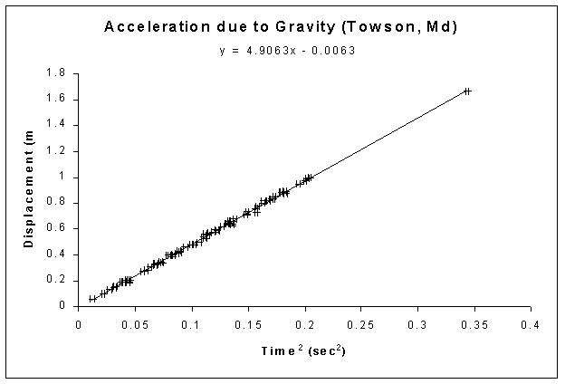
The results of an experiment by the Fall 2003 PHY542 class are
shown below. After dropping a mass from rest (vi
= 0) through vertical displacement h and measuring the travel
time, the data were plotted as h vs t2.
If the kinematic relationships are true, the slope of this curve
represents half of the acceleration due to gravity, ag.
A value of 9.81 m/s2 is within about 0.14% of the
accepted value in Towson.
Example with solution:
A ball is thrown from the street such that it rises past a 25m
high window ledge at 12 m/s. Find a) the velocity with which
it was launched, b) the maximum altitude above the street it
reaches, c) how long ago it was thrown, and d) the time until it
returns to the ground. Click here
for solution.
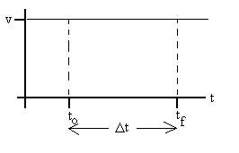
Let's break the time interval up into an infinite number of
infinitely small time intervals, dt, so that the velocity
is essentially constant over each.
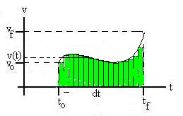
Then the displacement over each interval, dx, is v(t)
dt, and the total displacement should be the sum
(now, integral) of all the dxs
Dx =  dx
= titf
v(t) dt.
dx
= titf
v(t) dt.
Graphically, this integral is interpreted as the area under the
v(t) curve between times ti and tf
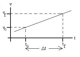
Here is a quick example:
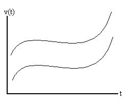
Each of the two curves shown will generate the same acceleration
curve, since the slopes of the two are the same for each value of
time, t. So, given a particular acceleration curve, it would
be impossible for one to determine which of an infinite number of
possible velocity curves it was derived from.
More mathematically, we see that Dv =  dv = titf a(t) dt.
Let's look at another situation:
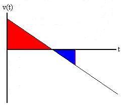
In this case, the velocity starts out positive, but there is a
negative acceleration (slope of the line). Eventually, the
velocity becomes zero and the object comes momentarily to rest,
having traveled through a displacement represented by the area
under the curve (the red area). As time progresses, we see
that the velocity becomes negative, the object reverses direction,
and we would expect that it may well arrive back at its starting
point, for a total displacement of zero. How does this play
out on the graph? Since displacement is basically velocity
times time interval, negative velocities result in negative
incremental displacements which are represented here by negative
area (blue). So, in this example, when the positive (red)
area above the axis equals the negative (blue) area under the
axis, the total displacement will be zero and the object will have
returned to its starting point.
Consider a mass oscillating on a spring:
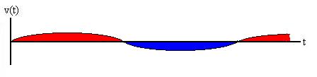
Once again, when the area 'under' the curve adds to zero, the
object has returned to its starting point.
Ball dropped from a rising helicopter (see Problem 2-8):
Many students believe that the ball begins to descend immediately
upon its release from the rising helicopter. This is not
so. Try lifting a pen upward with your hand palm down,
releasing it as it passes some point on the wall. If that
notion is correct, the pen will never appear above that spot on
the wall, but you will see that it does indeed continue to
rise. For some reason, it's easier to believe when you push
the pen with palm upward, so be sure to hold palm downward to more
closely simulate the scenario in the problem. Graphically,
we see
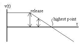
We see at first the constant velocity experienced while the ball
is still connected to the helicopter. At the release time,
the acceleration becomes -9.8 m/s2, as shown by the
negative slope of the line. A short time later, the velocity
is still positive, although less than it was, but a positive
velocity still means that the object is rising, and it will
continue to do so until the velocity reaches zero at the highest
point in the trajectory.
Speaking of that highest point, what is the acceleration at that
point? It is common to assume that it is zero, but that
confuses that velocity with the acceleration. We can look at
the graph above and see that the slope of the v(t) graph when v =
0 is still -9.8 m/s2. Or, think opf the velocity
just before the peak (positive) and just after the peak (
negative); the acceleration measures the change in velcoity, which
became more negative in that time interval. Or think of it
this way, since acceleration is related to the change in velocity,
if ag were zero at the peak, what would the object
do? No acceleration implies no change in velocity, so the
object would just hang in space, an event counter to our
experience.
This integrates to 1/2 vx2 + 1/2 vy2 + 1/2 vz2 , which becomes with the help of the Pythagorean theorem 1/2 (vx2 + vy2 + vz2) = 1/2 v2.